The armchair quantum physicist

We use Python Qutip to replicate the experiment performed by Alain Aspect and co-workers in 1982 (Ref 1), where for the first time the violation of Bell’s inequalies was experimentally demonstrated. The exact formulation of the inequality differs slighly from the original Bell inequality and is also known as the ‘CHSH inequality’. The paper by Clauser and Horne (Ref 2) provides background to the exact formulation of the Bell inequality used by Aspect. A lot has been said and written about Bell’s inequality, local theories, quantum mechanics, … a nice overview with a strong link to experimental set-up, history and interpretation is given by Mitchell (Ref 3).

1. Aspect, Dalibard and Roger, “Experimental test of Bell’s inequalities using time-varying analyzers,” Phys.Rev. Letter 49, 1802, December 1982
2. Clauser and Horne, “Experimental consequences of objective local theories,” Phys.Rev.D. 10 (2):536, July 1974
3. Dehlinger and Mitchell, “Entangled photons, nonlocality, and Bell inequalities in the undergraduate laboratory,” Am. J. Phys. 70 (9), 904, September

If you want to experience this Nobel prize winning experiment yourself by using some simple Python code check the Jupyter Notebook for Experimental test of Bell’s inequality on Github pages.

The Alain Aspect experiment

The Alain Aspect experiment looks deceptively simple. There is a light source and two detection stations. At each detection station the detectors can be set to detect one of two parameters. For instance detector at station 1 could detect parameter a or a’, and at station two we would detect parameter b or b’. In total there are four combinations for the two detection station (they could be set to detect ab, a’b, ab’ or a’b’). In practice setting the detectors is done by making them detect photon at a certain polarization angle, but for the actual conclusion from the experiment this is not relevant. Let’s bring this experiment closer to day-to-day live and compare to a simple game… (of course, any ‘game’ to mimic a physics experiment feels a bit artificial, the purpose is for explaining, not to be fun to play).

The game

Imagine playing a game with two players and a ‘dealer’. The dealer has 4 coins, for instance, two 2-euro coins and two 1-euro coins (any other currency will do). At each turn, the dealer gives one 2-euro and one 1-euro coin to each of the players, but hidden under a beaker such that the players cannot see them. The players decide individually whether they will look at the 2-euro coin or the 1-euro coin. After that decision, they look at the coins and note whether, for the coin of their choice, they see ‘heads’ or ‘tails’.

The dealer will ensure that over the game there are as many turns where a coin is ‘head’ as turns where a coin is ‘tail’, and the players have to select the 2-euro coin as often as they select the 1-euro coin.

The agreement is that if the two players select the same coin, they gain 1 euro if their outcome is equal. If they have different outcomes they have to pay. Also if player A selects the 2-euro coin and player B the 1-euro coin they win if they get an equal outcome. But (and here is the twist) if player A selected the 1-euro coin and player B the 2-euro coin they only win when they have a different outcome and have to pay when they have the same outcome.

So the rules of the game look like this:

Player A selects	Player B selects		Outcome equal	Outcome different
2-euro	2-euro		Gain 1 euro	Lose 1 euro
2-euro	1-euro		Gain 1 euro	Lose 1 euro
1-euro	2-euro		Lose 1 euro	Gain 1 euro
1-euro	1-euro		Gain 1 euro	Lose 1 euro

Now, we realize that the dealer has a large influence on the total win of loss for the players:

• Random dealer: if the dealer were to set up the turns completely randomly the players would have an equal likelihood to lose or to win. Independent of their choices the outcome could be equal or different.
• Nice dealer: if the dealer would be nice to the players he could select a strategy where always all coins are head, or all coins are tails. He should still randomly vary turn by turn whether he gives every player the coins head up, or tails up, but as long as in every turn both players get the same they would on average win 50 cents per game.
• Nasty dealer: a nasty dealer could follow a strategy where he always gives ‘all heads’ to one player and an ‘all tails’ to the other, leading to an average loss of 50 cents per game.

How could the players increase their wins above 50 cents per game? If they could communicate between themselves or with the dealer it would be possible. They could for instance agree to always look at the same coin, or they could let the dealer know beforehand which coins they will look at. Also, they could agree that the dealer can still change the values of the coins for player B after player A has made his move and observed the coins. In all these cases a strategy leading to a win of more than 50 cents per game is possible. However, it can be proven that when no information can be exchanged between the players and when the values of the coins are determined by the dealer irrespective of the choices of the players the gain is maximized to 50 cents per game. These assumptions are called ‘local realism’.

Now enter quantum mechanics. In quantum mechanics, the dealer is allowed to prepare the coins in such a way that they can be ‘head’ or ‘tail’ at the same time. Only when a player looks at the coins the real value of the coin is determined. Also, the dealer can create ‘entanglement’ between the coins. In that case, all coins are ‘head’ or ‘tail’ at the same time, but if one of the coins is detected by a player all coins instantaneously turn into a pre-defined ‘head’ or ‘tail’. This violates the principle of local realism as the impact of detecting a coin by Player A immediately affects what is observed by Player B.

The experiment

The experiment to first demonstrate this was performed by Alain Aspect and co-workers in 1982, and the groundwork was done by John Clauser and co-workers in 1974. Alain Aspect used photons that were sent from a source to two detectors. Just as our players in the game had to select a coin, the detectors in the experiment had to select between two polarization detectors (a or a’ for the detector on one side and b or b’ for the detector on the other side). For each combination of detector settings you can then express the correlation (P) as +1 if you measure the same outcome, and -1 if you measure opposite outcomes.

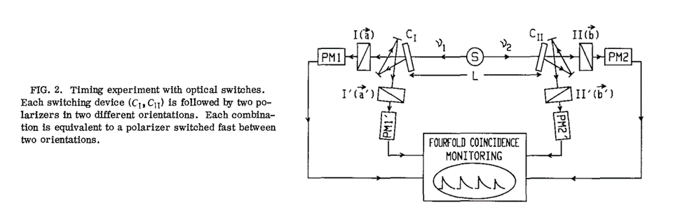
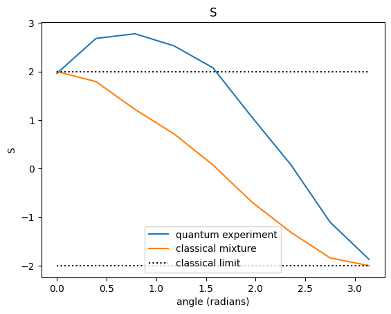
This experiment is very similar to our game. The photon source serves as the dealer. At both sides we find a detector acting as a player. The detectors can be set to measure in two different ways, denoted by a and a’ for detector 1. For detector 2 the options are to detect in setting b or b’. This is equivalent to the players choosing to observe the 1-euro coin or the 2-euro coin. The choices of the players/detectors lead to four different situations. In three of these there is a ‘reward’ for having a high correlation (the more the results are the same, either detecting a photon or detecting heads/tails, the higher the score). The twist is that for one of the situations the reward is given for a high anti-correlation (the more you find opposite results the higher the score). In the game the reward was expressed in euro’s, in the experiment we define the parameter S= Pab + Pa’b – P ab’ +Pa’b’. Here Pxy is the correlation for detector setting ‘x’ and ‘y’. Just as in our game the average pay off was always between +50cnts and -50cnts, in the experiment the value for S is always between -2 and 2 (based on the underlying assumptions for ‘local realism’).

Theoretically quantum mechanics allows violation of this ‘local realism’. There could be entanglement and the results of measurement at detector 1 could travel (fast than light) to detector 2 to influence the outcome of the measurement. This ‘spooky action at a distance’ was heavily debated and for some a reason to belief quantum mechanics was ‘ incomplete’ . It is therefore difficult to overstate the importance of the actual experiment. Either the experiment would proof quantum mechanics wrong (creating the need for a new fundamental theory), or the experiment would proof quantum mechanics right, violating very basic assumptions related to reality and locality.

As we all know, the experiment proved quantum mechanics right and the sceptics wrong. There is ‘ spooky action at a distance’. The fun thing is that nowadays very accessible tools are available to experience this ourselves. To model the Aspect experiment in Python you can check out the Jupyter Notebook( https://robhendrik.github.io/Bell-test-simulation/) where below graph is made. The parameter S on the vertical axis is exactly the ‘S’ used above. We see that if we run a quantum experiment for certain settings of the detectors (i.e., for a given angular alignment) this S goes beyond the classical limits. If we do the same experiment with a classical mixture we get the same result as for our coin game and limit ‘S’ to values between -2 and 2.

It is quite exciting that you can nowadays from your lazy armchair perform the very quantum experiments which shocked the world, and which triggered questions to which today we do not have the full answer.