Simulating the HOM effect on a quantum computer

See the Jupyter Notebook for this post on Github pages. This contains all code and details related to this post.

This is the third post from a series of three on the HOM effect. For the first post see Beamsplitters and the quantum HOM effect . For the second post see The HOM effect explained.

Main reference: C. K. Hong, Z. Y. Ou, and L. Mandel, “Measurement of subpicosecond time intervals between two photons by interference”, Phys. Rev. Lett. 59, 2044 – Published 2 November 1987

Introduction

Posts about the beamsplitter and the quantum HOM effect

In our first post we demonstrated the quantum HOM effect in computer simulation using Python QuTiP. We see that if two ‘indistinguishable’ photons enter two different input ports of a beamsplitter they somehow always come out in the same port and never each in a different port. We showed how we can tune this effect by varying the level of ‘indistinguishability’, for instance through changing the polarization of the photons from being parallel to eachother to being orthogonal to eachother.

In the second post we use quantum mechanics to describe the HOM effect. If there are multiple ways to get to the same result these ‘paths’ can experience quantum interference. In the case of the HOM effect we can have the two photons at different output ports if they both are transmitted, or if they both are reflected. These two different paths lead to the same measurement outcome. Quantum interference suppressed this outcome because the two paths have amplitudes with opposite sign, so they cancel eachother out.

On this third post we simulate the HOM effect on a real quantum computer. There is no real quantum advantage, so the simulation does not lead to new insights on the physics of the HOM effect. It does however serve as a nice demonstration for modelling a physical system such that it can be simulated.

The HOM effect

In this post we use a very simple optical component: A beamsplitter. This beamsplitter has two input ports and two output ports. For single photons we find the expected, and rather boring outcome that the photon either passes through the beamsplitter, or is reflected by the beamsplitter with a probability depending on the reflectance or transmittance of the beamsplitter. For a 50%/50% beamsplitter you would find an input photon with equal likelihood in any of the output ports of the beamsplitter.

However, when using two photons it gets a lot more interesting. We see that when the photons enter into different ports and are fundamentally ‘indistinguishable’ an effect occurs leading to the two photons always being together in any of the outputs. This ‘bunching’ is known at the HOM effect, named after Hong, Ou and Mandel (see their paper “Measurement of subpicosecond time intervals between two photons by interference” which mentioned in the references for this notebook)

To model the beamsplitter we define the matrix below. Here the transmission coefficient is $t$ and the reflection coefficient is $r$ . These coefficients act on the ampitudes of the electric field. The probability for photons to be transmitted or reflected is the square of the absolute value of these amplitudes. So transmission probability is $|t|^{2}$ and reflection probability is $|r|^{2}$ . If for instance $t = r = \frac{1}{\sqrt{2}}$ the probability for a single photon to be reflected is $r^{2} = \frac{1}{2}$ and the probability to be transmitted is $t^{2} = \frac{1}{2}$ . So this would be a 50%/50% beamsplitter equally splitting the light between the output ports. The matrix describing the general beamsplitter is

$\begin{pmatrix} r & t \\ t & -r \\ \end{pmatrix}$

For the 50%/50% beamsplitter the matrix looks like

$\begin{pmatrix} \frac{1}{2} \sqrt{2} & \frac{1}{2} \sqrt{2} \\ \frac{1}{2} \sqrt{2} & -\frac{1}{2} \sqrt{2} \\ \end{pmatrix} = \frac{1}{2} \sqrt{2} \begin{pmatrix} 1 & 1 \\ 1 & -1 \\ \end{pmatrix}$

For more information on how to describe a beamsplitter with a matrix check out wikipedia or the tutorial on the site of John Howell.

To describe the light we use Fock states (see wikipedia). In a Fock state there is a well defined amount or photons in each channel. So if we look at the two input ports of the beamsplitter we could have state $|00>$ with zero photons in either input, or we could have state $|21>$ with 2 photons in one port and one photon in the other port. The HOM effects is such that if we have input state $|11>$ (one photon in each input) we measure output states $|02>$ and $|20>$ with 50% probability each. We never measure $|11>$ at the output.

Transition matrices from beamsplitter input to output for multi-photon states (Fock states)

For the beamsplitter we have two input channels and two output channels. When using Fock states the beamsplitter ‘transforms’ input state $|nm>$ into output state $|uv>$ . Here $n$ and $m$ are the number of photons in input channels 1 and 2, and $u$ and $v$ are the number of photons in output channels 1 and 2. We can make a transition matrix describing how this transformation happens. This matrix will have for instance a coeffient at indices ’10’ and ’01’ which indicates the amplitude for the transition from input state $|10>$ to output state $|01>$ . If this amplitude is for instance $\frac{1}{\sqrt{2}}$ the probability to end up in state $|01>$ would be $(\frac{1}{\sqrt{2}})^{2}$ or $\frac{1}{2}$ .

As we deal with a lossless beamsplitter the total amount of photons in the input and output have to be the same (this is the law of conservation of energy, we cannot create photons out of nothing and without loss they can also not disappear). So an input state with one photon ( $|10>$ or $|01>$ ) can only transform to an output state with one photon ( $|10>$ or $|01>$ ). The total probability should be 100%. So if we know that the probability to go from input $|10>$ to output $|01>$ is $\frac{1}{2}$ we automatically know that the probability to from input $|10>$ to output $|10>$ is also $\frac{1}{2}$ . We also know that the probability to go from input $|10>$ to for instance output $|10>$ , $|11>$ or $|20>$ is zero as the total number of photons is not kept the same.

The transition matrix contains amplitudes and the transition probability is the square of the absolute value of the amplitude. The probability is a real number ranging from 0 to 1. The amplitude can be a complex number. We need to calculate with amplitudes to be able to include quantum interference where a probability is reduced due to two amplitudes cancelling eachother for the different ways to get to an component. As explained in ithe previous post this is the basis for the HOM effect. If we would ignore the amplitude and only calculate with probabilities we would not be able to describe the interesting quantum effects.

Below we define the Python function to calcute the Fock state transition matrix. Here $r$ and $t$ are reflection and transmission amplitudes. For the 50%/50% beamsplitter we take $t = r = \frac{1}{\sqrt{2}}$ . The name for this function in our Python code is:

create_Fock_coefficients(r, t, make_unitary)

If the paramater ‘make_unitary’ is set to ‘False’ we use the transition coefficients defined by the physical system. This leads to a practical issue when modelling. To keep the size of the model finite we have to set a maximum to the number of photons per channel. We do this by setting the parameter ‘length_of_fock_state’. If set this to for instance 3 the maximum photon count per channel is 2 (we have 3 options per channel, either 0,1 or 2 photons).

If we limit the photon count per channel to for instance 2, we can have input state $|22>$ . This means the output state could be $|31>$ or $|40>$ , with photon count per channel that is higher than the earlier set value of 2. But if we extend the basis to include this and allow photon count of 4 per channel the input could be $|44>$ and the output should include $|80>$ . We can of course have a different basis as input and output, but that is not practical. Also the system would not be ‘reversible’ which poses an issue later if we want to model on a quantum computer. So for practical purposes we can set the option ‘make_unitary’ to ‘True’. In that case the coefficients will be articially set if the total photon count at either input or output is above the maximum defined. So for a maximum photon count per channel set to 2 and ‘make_unitary’ set to ‘True’ the transition from $|21>$ to $|21>$ will be artificially set to 1 and the transition from $|21>$ to $|03>$ will be zero (so we can leave state $|03>$ out of consideration). This is not the real physics. A real beamsplitter will have a probability to go from $|21>$ to $|03>$ . Purely from practical purposes we exclude this. For total photon counts up to 2 the matrix will describe the real system, for higher counts the matrix is artificial and does not describe the real system with ‘make_unitary’ set to ‘True’.

Below the two transition matrices for the physical system with ‘make_unitary’ equal to ‘False’. In some rows and columnesn(for $|21>$ , $|12>$ and $|22>$ ) the squares of the amplitudes do not add up to 1.

r = t = 1/math.sqrt(2)
make_unitary = False
Fock_coefficients = create_Fock_coefficients(r, t, make_unitary)

      00    01    02    10    11    12    20    21   22
00  1.0  0.00  0.00  0.00  0.00  0.00  0.00  0.00  0.0
01  0.0  0.71  0.00  0.71  0.00  0.00  0.00  0.00  0.0
02  0.0  0.00  0.50  0.00  0.71  0.00  0.50  0.00  0.0
10  0.0 -0.71  0.00  0.71  0.00  0.00  0.00  0.00  0.0
11  0.0  0.00 -0.71  0.00  0.00  0.00  0.71  0.00  0.0
12  0.0  0.00  0.00  0.00  0.00 -0.35  0.00  0.35  0.0
20  0.0  0.00  0.50  0.00 -0.71  0.00  0.50  0.00  0.0
21  0.0  0.00  0.00  0.00  0.00 -0.35  0.00 -0.35  0.0
22  0.0  0.00  0.00  0.00  0.00  0.00  0.00  0.00 -0.5

When we model with with

make_unitary = True

we artificially set the transition for states with in total more than two photons to 1, and the it becomes a ‘nice’ transition matrix.

r = t = 1/math.sqrt(2)
make_unitary = True
Fock_coefficients = create_Fock_coefficients(r, t, make_unitary)

     00    01    02    10    11   12    20   21   22
00  1.0  0.00  0.00  0.00  0.00  0.0  0.00  0.0  0.0
01  0.0  0.71  0.00  0.71  0.00  0.0  0.00  0.0  0.0
02  0.0  0.00  0.50  0.00  0.71  0.0  0.50  0.0  0.0
10  0.0 -0.71  0.00  0.71  0.00  0.0  0.00  0.0  0.0
11  0.0  0.00 -0.71  0.00  0.00  0.0  0.71  0.0  0.0
12  0.0  0.00  0.00  0.00  0.00  1.0  0.00  0.0  0.0
20  0.0  0.00  0.50  0.00 -0.71  0.0  0.50  0.0  0.0
21  0.0  0.00  0.00  0.00  0.00  0.0  0.00  1.0  0.0
22  0.0  0.00  0.00  0.00  0.00  0.0  0.00  0.0  1.0

An alternative approach would be to limit the set of input and output states only to a specific set (i.e., only look at states with up to 2 photons and exclude the rest). However, when modelling with a register of (qu)bits it is convenient to have a number of states that is a power of 2. So we can easily deal with a basis of 2, 4, 8 or 16 states, but have to take specific care when dealing with for instance a basis consisting of 6 states. Right now we have nine states, so the next step is to condense to 8 states by removing one of the states with total number of photons larger than 2 (for those states we anyway have set the transition amplityde articificially to 1, so there is no physical meaning to it).

Mapping the photons states onto qubit states

In this notebook we want to model the HOM effect on ultimately a real quantum computer. This means we need to map the Fock states discussed above on a (qu)bit state. Above transition matrix has a basis of 9 states. So we would need 4 bits, with $2^{4} = 16$ states. As we know that some states in the Fock state basis are artificially set anyway we can also limit the basis to 8 states and use a register of 3 (qu)bits.

Anyway we will need a mapping table where we map a Fock state on a qubit register. This is a choice we make. There is no physics prescribing whether we map for state $|01>$ on qubit state ‘001’ or ‘100’.

Let’s take the simplest approach and follow the ordering of basis states implemented in Python QuTiP anyway. We look at how the Fock states are mapped on the QuTiP bases state and we look at how the qubit states are mapped.

create_lookup_Fock_states(length_of_fock_state, no_of_channels)
create_lookup_QubitCircuit_states(number_of_qubits)

If we ignore the 9th state in the Fock state basis (which we do not intend to use anyway, and already did set to an artificial transition coefficient to make the matrix unitary) we can keep the order of the basis and come to the mapping defined as below.

merge_lookups(map, first_lookup, second_lookup)

Lookup table from Fock states to Qubits
Fock states <==> QubitCircuit qubits
|00>  <==> 000
|01>  <==> 001
|02>  <==> 010
|10>  <==> 011
|11>  <==> 100
|12>  <==> 101
|20>  <==> 110
|21>  <==> 111

With this mapping we can define the transition matrix between qubit states to model the beamsplitter (and model the HOM effect)

Transition matrix between registers of 3 qubits. 
This matrix models the transition between Fock states in 2 channels, with total photon count of maximum 2

     000   001   010   011   100  101   110  111
000  1.0  0.00  0.00  0.00  0.00  0.0  0.00  0.0
001  0.0  0.71  0.00 -0.71  0.00  0.0  0.00  0.0
010  0.0  0.00  0.50  0.00 -0.71  0.0  0.50  0.0
011  0.0  0.71  0.00  0.71  0.00  0.0  0.00  0.0
100  0.0  0.00  0.71  0.00  0.00  0.0 -0.71  0.0
101  0.0  0.00  0.00  0.00  0.00  1.0  0.00  0.0
110  0.0  0.00  0.50  0.00  0.71  0.0  0.50  0.0
111  0.0  0.00  0.00  0.00  0.00  0.0  0.00  1.0

Above matrix is important for what follows. This is the matrix containing the transition amplitudes between the qubit states which we want to achieve with out quantum circuit. If we know the quantum circuit establishes this transition, we also know the circuit is modelling the beamsplitter and the HOM effect.

Building a quantum quantum circuit that simulates the HOM effect

We use Qiskit to create a quantum circuit that simulates the beamsplitter. The circuit will have three qubit and three classical bits (to store the measurment results). We have a helper function to cycle through all input states in our lookup table and determine the probability of the various outcomes. This function is:

get_all_probabilities(circuit, lookup_table)

We also define a helper function to plot the unitary matrix of the quantum circuit .

print_circuit_unitary(circuit, lookup_table)

Now we are ready to build the quantum circuit. In a first approach we create a custom gate which exactly contains the transition matrix defined before as

qubit_transition_matrix

We then build a circuit with just this one gate, which contains this transition matrix as ‘operator’. This is of course a custom gate and not part of any standard library.

circuit.unitary(Operator(qubit_transition_matrix), circuit.qubits, label='HOM simulation')

The circuit with this custom gate looks like this (just one gate):

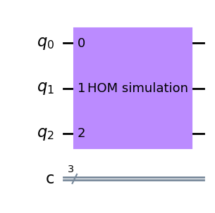
This quantum circuit should simulate the HOM effect. We indeed get the expected outcome when running the circuit. So we are capable of simulating the beamsplitter on a quantum circuit, but have to use a ‘custom’ gate to do so.

Input Fock state: |00> (qubit |000>)
---- Outcome Fock state: |00> (qubit |000>) with probability 100%
Input Fock state: |01> (qubit |001>)
---- Outcome Fock state: |10> (qubit |011>) with probability 49%
---- Outcome Fock state: |01> (qubit |001>) with probability 51%
Input Fock state: |02> (qubit |010>)
---- Outcome Fock state: |02> (qubit |010>) with probability 25%
---- Outcome Fock state: |11> (qubit |100>) with probability 50%
---- Outcome Fock state: |20> (qubit |110>) with probability 24%
Input Fock state: |10> (qubit |011>)
---- Outcome Fock state: |10> (qubit |011>) with probability 50%
---- Outcome Fock state: |01> (qubit |001>) with probability 50%
Input Fock state: |11> (qubit |100>)
---- Outcome Fock state: |02> (qubit |010>) with probability 50%
---- Outcome Fock state: |20> (qubit |110>) with probability 50%
Input Fock state: |12> (qubit |101>)
---- Outcome Fock state: |12> (qubit |101>) with probability 100%
Input Fock state: |20> (qubit |110>)
---- Outcome Fock state: |11> (qubit |100>) with probability 50%
---- Outcome Fock state: |02> (qubit |010>) with probability 26%
---- Outcome Fock state: |20> (qubit |110>) with probability 23%
Input Fock state: |21> (qubit |111>)
---- Outcome Fock state: |21> (qubit |111>) with probability 100%

If we then check the unitary matrix for the total circuit we see indeed the correct results

      000   001   010   011   100  101   110  111
000  1.0     .     .     .     .    .     .    .
001    .  0.71     . -0.71     .    .     .    .
010    .     .   0.5     . -0.71    .   0.5    .
011    .  0.71     .  0.71     .    .     .    .
100    .     .  0.71     .     .    . -0.71    .
101    .     .     .     .     .  1.0     .    .
110    .     .   0.5     .  0.71    .   0.5    .
111    .     .     .     .     .    .     .  1.0

So this is not very exciting. We have simply created a custom gate by using the transition coefficients between the different Fock states and by using a lookup table mapping the Fock states on the qubit states. However, with this infrastructure setup we can now try to build a quantum circuit from more standard gates to come to the same result.

Simulate the HOM effect with a quantum circuit using ‘standard’ gates.

We want to create a quantum circuit to simulate the beamsplitter and the HOM effect using standard gates. The goal is to create the same unitary matrix as we had from the custom gate defined in previous section. Obviously there are automated functions available to do this (like Qiskit transpile), but is insightfull to try by hand. An easy and step-by-step way to resolve this manually is to start from the custom gate and then extend with standard gates to turn the matrix into the identity matrix. So we want to get to $I = M \cdot Gate_1 \cdot Gate_2 \cdot Gate_3 \ldots$ (where $I$ is the identity matrix, $M$ the custom unitary and $Gate_i$ a standard gate). So we add gates to the custom gate to create a circuit which does nothing. We then know that the added gates are the reverse of the custom gate, and that reversing the added standard gates should replicate the custom gate. So in formulas this looks like:

$\begin{array}{lcl} I & = & M \cdot M^{-1} \\ I & = & M \cdot Gate_1 \cdot Gate_2 \cdot Gate_3 \ldots Gate_{n-1} \cdot Gate_n \\ M^{-1} & = & Gate_1 \cdot Gate_2 \cdot Gate_3 \ldots Gate_{n-1} \cdot Gate_n \\ M & = & (Gate_1 \cdot Gate_2 \cdot Gate_3 \ldots Gate_{n-1} \cdot Gate_n)^{-1} \\ M & = & Gate_n^{-1} \cdot Gate_{n-1}^{-1} \ldots Gate_3^{-1} \cdot Gate_2^{-1} \cdot Gate_1^{-1} \end{array}$

We start by taking unitary matrix which comes from our ‘custom’ gate

circuit.unitary(Operator(qubit_transition_matrix), circuit.qubits, label='HOM simulation')

This is the orginal ‘custom gate’

      000   001   010   011   100  101   110  111
000  1.0     .     .     .     .    .     .    .
001    .  0.71     . -0.71     .    .     .    .
010    .     .   0.5     . -0.71    .   0.5    .
011    .  0.71     .  0.71     .    .     .    .
100    .     .  0.71     .     .    . -0.71    .
101    .     .     .     .     .  1.0     .    .
110    .     .   0.5     .  0.71    .   0.5    .
111    .     .     .     .     .    .     .  1.0

The idea is now to add gates after this custom gate to ulimately get to the identity transformation. We can start by removing the mixing between states ‘001’ and ‘011’. We do this by first setting the ‘most significant’, or left qubit from 0 to 1 by an ‘NOT’ operation, or ‘X’ operation on qubit 2 (‘circuit.x(2)’). So we have the states ‘101’ and ‘111’. We then apply the controlled Hadamard gate with bits 0 and 2 as controls, and bit 1 (the middle qubit) as target. Then we flip back qubit 2 by another ‘NOT’ operation.

circuit.x(2)
circuit.unitary(CCH, [q[1], q[0], q[2]], label='CCH')
circuit.x(2)

The resulting transition matrix indeed shows that we have removed the mixing between states ‘001’ and ‘011’ and have made the matrix more diagonal.

      000  001   010  011   100  101   110  111
000  1.0    .     .    .     .    .     .    .
001    .  1.0     .    .     .    .     .    .
010    .    .   0.5    . -0.71    .   0.5    .
011    .    .     . -1.0     .    .     .    .
100    .    .  0.71    .     .    . -0.71    .
101    .    .     .    .     .  1.0     .    .
110    .    .   0.5    .  0.71    .   0.5    .
111    .    .     .    .     .    .     .  1.0

We see that for states ‘001’ and ‘011’ the matrix has simplified and these states only transition to themselves. The idea is to continue until we have all 1’s on the diagonal. Let’s remove the factor ‘0.5’ and ‘-0.5’ for states ‘010’ and ‘110’. For this we set qubit zero to value 1, then apply the controlled Hadamard gate with qubit two as target and qubits zero and one as control. Then as last step we flip back qubit zero.

circuit.x(0)
circuit.unitary(CCH, [q[2], q[0], q[1]], label='CCH')
circuit.x(0)

And indeed, if we look at the resulting transition matrix it has further simplified and has become more ‘diagonal’.

      000  001   010  011  100  101   110  111
000  1.0    .     .    .    .    .     .    .
001    .  1.0     .    .    .    .     .    .
010    .    .  0.71    .    .    .  0.71    .
011    .    .     . -1.0    .    .     .    .
100    .    .  0.71    .    .    . -0.71    .
101    .    .     .    .    .  1.0     .    .
110    .    .     .    . -1.0    .     .    .
111    .    .     .    .    .    .     .  1.0

A few more steps to get to a fully diagonal matrix.

circuit.x(0)
circuit.toffoli(2,0,1)
circuit.unitary(CCH, [q[2], q[0], q[1]], label='CCH')
circuit.x(0)

      000  001  010  011  100  101  110  111
000  1.0    .    .    .    .    .    .    .
001    .  1.0    .    .    .    .    .    .
010    .    .  1.0    .    .    .    .    .
011    .    .    . -1.0    .    .    .    .
100    .    .    .    . -1.0    .    .    .
101    .    .    .    .    .  1.0    .    .
110    .    .    .    .    .    .  1.0    .
111    .    .    .    .    .    .    .  1.0

Basically we are there, but to get to the full identity matrix let’s also remove the minus sign for states ‘011’ and ‘100’

circuit.cnot(control_qubit=2, target_qubit=0)
circuit.cnot(control_qubit=2, target_qubit=1)
circuit.cp(math.pi, control_qubit=0, target_qubit=1)
circuit.cnot(control_qubit=2, target_qubit=0)
circuit.cnot(control_qubit=2, target_qubit=1)

     000  001  010  011  100  101  110  111
000  1.0    .    .    .    .    .    .    .
001    .  1.0    .    .    .    .    .    .
010    .    .  1.0    .    .    .    .    .
011    .    .    .  1.0    .    .    .    .
100    .    .    .    .  1.0    .    .    .
101    .    .    .    .    .  1.0    .    .
110    .    .    .    .    .    .  1.0    .
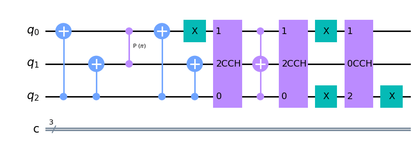
111    .    .    .    .    .    .    .  1.0

We now have added standard gates to our custom gate to get to the identity matrix. So we show that the circuit below is such that for each input state the output is equal to the input. The total circuit looks like this. The ‘barriers’ are placed inbetween the different steps for visualization.

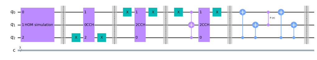
We can simplify this by removing the barriers and the sequence of 2 NOT’s for qubit zero.

By inverting this sequence of standard gates that come after the custom gate we can decompose our custom gate into standard gates. We then get this circuit to do the same as our custom gate. So this circuit simulates the beamsplitter and the HOM effect.

Decompose the quantum circuit to remove the 3-qubit gates

The disadvantage of our circuit is that it contains double controlled gates. We can easily replace them by single controlled gates using the right decomposition. First we decompose the double controlled Hadamard gate. The sequence below has exactly the same effect as the double controlled Hadamard gate.

gate = XGate().power(1/2).control(1)


circuit_CCX = QuantumCircuit(3)
circuit_CCX.append(gate, [1,0])
circuit_CCX.cnot(target_qubit=1, control_qubit=2)
circuit_CCX.append(gate.inverse(), [1,0])
circuit_CCX.cnot(target_qubit=1, control_qubit=2)
circuit_CCX.append(gate, [2,0])
circuit_CCX.draw('mpl')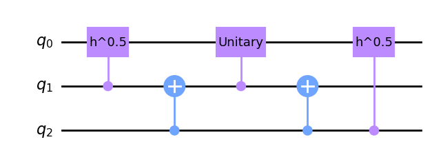

Then we decompose the Toffoli gate, or double controlled NOT gate into only 2-qubit gates. The sequence below has exactly the same effect as the Toffoli gate.

gate = XGate().power(1/2).control(1)


circuit_CCX = QuantumCircuit(3)
circuit_CCX.append(gate, [1,0])
circuit_CCX.cnot(target_qubit=1, control_qubit=2)
circuit_CCX.append(gate.inverse(), [1,0])
circuit_CCX.cnot(target_qubit=1, control_qubit=2)
circuit_CCX.append(gate, [2,0])
circuit_CCX.draw('mpl')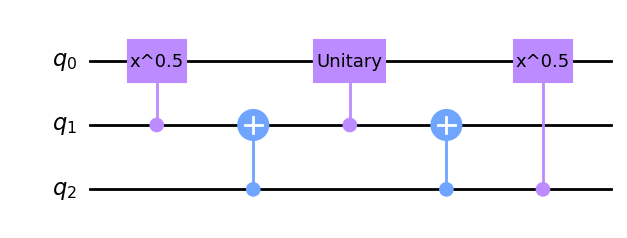

We can replace the double controlled gates in our circuit by their decomposition and arrive to below circuit to model the beamsplitter with only 2 qubit gates.

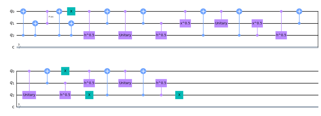
To check whether it works we can look at the unitary matrix describing this circuit. It is still the same unitary as we started with. So the decomposition from custom gate to standard gates to 2-qubit gates has not affected what the circuit does. It is still the same transition from input states to output states.

     000   001   010   011   100  101   110  111
000  1.0     .     .     .     .    .     .    .
001    .  0.71     . -0.71     .    .     .    .
010    .     .   0.5     . -0.71    .   0.5    .
011    .  0.71     .  0.71     .    .     .    .
100    .     .  0.71     .     .    . -0.71    .
101    .     .     .     .     .  1.0     .    .
110    .     .   0.5     .  0.71    .   0.5    .
111    .     .     .     .     .    .     .  1.0

Running the simulation on a quantum computer

Lets’ first summarize what we did so far:

We started this post by generating a ‘transition matrix’ which models the behavior of a beamsplitter, including the quantum HOM effect. Here we use Fock states as a basis. These states describe the number of photons in a channel.
We then created a mapping (a ‘lookup_table’) of the Fock states on a register of tree qubits. For these qubits we then generated a unitary transition matrix describing the physical mechanism in the beamsplitter. We had to do some tricks to keep the matrix unitary and the result is only physically valid for systems with 2 photons or less.
We then created a quantum circuit for3 qubits circuit and a single ‘custom’ gate. In our code the circuit is called ‘circuit_custom_unitary’. The custom gate was defined by the unitary matrix describing the transition between Fock states for our beamsplitter. With the propose mapping in the ‘lookup_table’.
We then manually decomposed the circuit by using three qubit gates (the double controlled Hadamard gate) and the double controlled NOT gate (aka Toffoli gate). This circuit is called ‘circuit_manual’ in our code.
We then as final step further decomposed the circuit by using only 2 qubit gates. The result is called ‘circuit_manual_2’.
All these circuits realize the same transformation from input to output states and ideally give the same outcome. As next step we will run these circuits on first a ‘fake’ quantum computer and then on a real quantum computer. We will see how the circuits differ in their sensitivity to noise.

Running the algorithm on a ‘fake’ quantum computer (a simulator)

Next we want to run our circuits on a quantum computer. We will do this by using the “IBM Quantum Lab” environment.

We run these circuits first on a simulated backend and compare the results to an ideal, noiseless, situation. For the noiseless reference we use Qiskit’s build in ‘AerSimulator’ as backend. We compare results to the ‘FakeLimaV2‘ backend.

Two different visualizations are used to compare the results. First we use a two-dimensional plot where the gray scale indicates the transition probability. Black is a 100% probability and white is 0% probability. We can compare how this picture looks for the noiseless simulation and for the simulations on the fake backend. We clearly see the white spots in the noiseless simulation disappear for the simulations on the fake backend. This illustrates the noise we have to deal with on a real quantum computer. Note that we used a non-linear scaling of the color bar to make the low noise values visible. We do also see that the result is best when using the custom gate as input. It gets worse if we use our ‘manually transpiled circuits’. The reason is that the circuit is transpiled anyway for optimal use on the backend and the algorithms in Qiskit are doing a better job at this than we did. Giving these algorithms the orginal circuit allows for more efficient optimization.

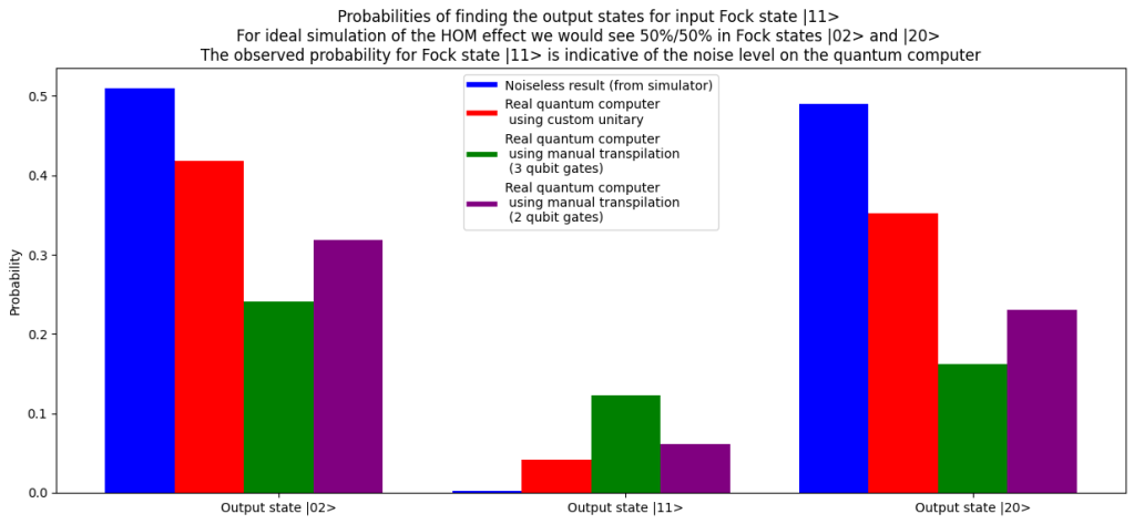
An alternative way to visualize the result is by looking at the HOM effect specifically: If we use $|11>$ as input state, do we see 100% outcomes in $|02>$ and $|20>$ or do we also see result in $|11>$ ? The more noise, the higher we expect the number of outcomes in the $|11>$ state (remember, the HOM effect is about surpressing the situation where we find the two photons behind separate output ports and only allowing outcomes where the photons bunch togeter behind one of the output ports of the beamsplitter. This is the effect we are simulating. So an ideal simulation would show no transition probability from the $|11>$ input state to the $|11>$ output state).

If we look at the result in below bar chart we see that, due to noise, the probability to end up in state $|11> is larger than zero. Still, we do see a nice contrast between the probabilities to end up in$ latex |02>$ or $|20>$ , so the noise has not completely overcome the simulated effect. This graph also confirms that we get the least noise when starting with the circuit based on the custom gate, and skip the manual transpilation.

Running the algorithm on a real quantum computer

Below the code we use to run the circuits on the IMB quantum backend. We use the ‘ibmq_lima’ device (see this link for documentation) and use Qiskit ‘runtime’ for execution. This part of the code we executed on the IBM server via IBM quantum Lab. This avoids complexity with SSL licenses and credentials.

We run the three circuits sequentially. As the waiting time can be up to a few days we fetch the results from the IMB dashboard. Once the circuits are defined in IBM quantum lab we use below code to run the circuits.

# First define a list of circuits to loop through the different input states

circuit_to_run = circuit_custom_unitary
#circuit_to_run = circuit_manual_2
#circuit_to_run = circuit_manual_2

backend = service.get_backend('ibmq_lima')
q = QuantumRegister(3,'q')
c = ClassicalRegister(3,'c')
initial_states = lookup_table.values()
list_of_circuits = []
for state in initial_states:
    circuit_in_list = QuantumCircuit(q,c)
    circuit_in_list.initialize(state, q)
    circuit_in_list.compose(circuit_to_run, [0, 1, 2], inplace=True)
    circuit_in_list.measure_all()
    transpiled_circuit = transpile(circuit_in_list, backend)
    list_of_circuits.append(transpiled_circuit)

# And then we submit the list or circuits for execution
from qiskit_ibm_runtime import (
    QiskitRuntimeService,
    Session,
    Sampler,
    Estimator,
    Options,
)
service = QiskitRuntimeService(channel="ibm_quantum")
options = Options(optimization_level=3, resilience_level=1)
sampler = Sampler(session=backend)
job = sampler.run(list_of_circuits)
print(job.job_id())

The results are fetched (after a few days) from the IBM site. We visualise the results just as we did with the results from the ‘fake’ backend. The two-dimensional grey scale shows the noise level. The left-most picture is the noisless simulation included for reference. Clearly we see the noise added by the quantum computer. We also see, just as predicted from our runs on the fake quantum computer, that the circuit based on the custom gate performs best.

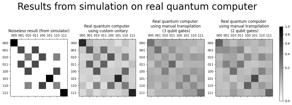
If we look at the quantum HOM effect specifically we can see how much the result on the real quantum computer shows that the outcome $|11>$ is suppressed. For all runs on the real quantum computer we see a non-zero probability to go from $|11>$ input to $|11>$ output, but especially for the circuit based on our custom gate there is a nice contrast between the high probability expected in the $|02>$ or $|20>$ and the low probability in the $|11>$ .

Conclusion

In this post we showed how to model a beamsplitter on a real quantum computer. As result we do see the expected statistics in photon counts at the output port. Specifically we see the HOM effect and the suppression of the outcome where two indistinguishable photons end up behind different ports. We do see that the photons like to ‘bunch’ together.

Realistically there is no added value in this simulation over the simulations done on a classical computer. We did not use an algorithm exploiting a quantum advantage. Still, being able to run a quantum simulation from home and getting sensible results is fun and insightfull, especially when the quantum computer is modelling a true quantum effect.

The armchair quantum physicist