The armchair quantum physicist

In previous posts we used Python to model and analyze quantum optical systems. We looked at the famous experiment by Alain Aspect (see experimental test of Bell’s inequality), we looked at three-photon entanglement in GHZ states (see Greenberger-Horne-Zeilinger entanglement), and we looked at the interesting phenomena in a simple beam splitter (Beam splitters and the quantum HOM effect). Now we present a Python module which makes modeling these quantum optical systems a lot easier: FockStateCircuits.

Check out GitHub for source code and supporting documentation.

Features

* Evaluate quantummechanical interaction between optical channels

* Easy to model famous experiments like Alain Aspects nobel prize winning experiment, the HOM effect, GHZ state generation as first demonstrator by Anton Zeilinger, quantum teleportation, …

* Optical and quantum channels combined to easily process a variety of input states

* Features for easy plotting and visualizing the circuits and the states

FockStateCircuit

‘FockStateCircuit’ is intended to model (quantum) optical quantum circuits where the different channels carry well defined number of photons (typically low numbers like 0,1,2,3, …). These states where the number of photons is well defined are called ‘Fock states’. The class supports optical channels where interaction is established through optical components, like beamsplitters or waveplates. Circuits can also contain classical channels. These can be used to store the result of a measurement or to set the behavior of optical componens.

FockStateCircuits run instances from the class ‘CollectionOfStates’. These are collections of states belonging to the FockStateCircuit. The states describe photon numbers in the optical channels and the values of the classical channels. When we run a collection of states on a circuit the collection will evolve through the circuit from an ‘input’ collection of states to an ‘output’ collection of states.

The states in the collections are instances of the class ‘State’. The states describe photon numbers in the optical channels and the values of the classical channels. The states also carry the history of the different measurement results during evolution through the circuit, as well as a reference to the initial state they originate from.

An initial example

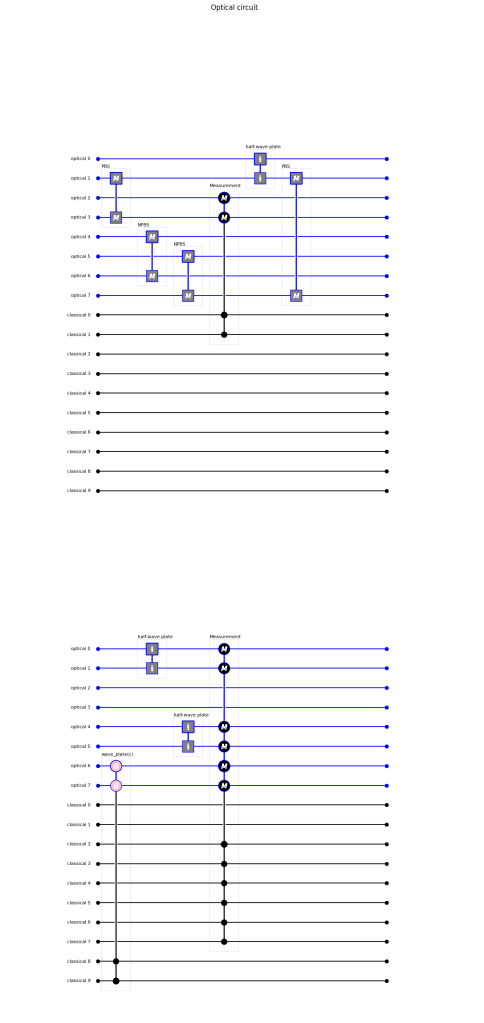
Below an example of a FockStateCircuit with 8 optical channels and 10 classical channels. The circuit has polarizing beamsplitters, non polarizing beamsplitters, wave plates and detectors. There is also a wave plate (indicated by ‘wave-plate(c)’) whose properties are set by the values in the classical channels.

A FockStateCircuit for the HOM effect

Let’s build a circuit to model the HOM effect. For this we look at a 50%/50% beamsplitter with two input ports and two output ports. The beamsplitter is polarization independent, so the splitting ratio does not depent on the polarization and the components does not change the polarization of the light.

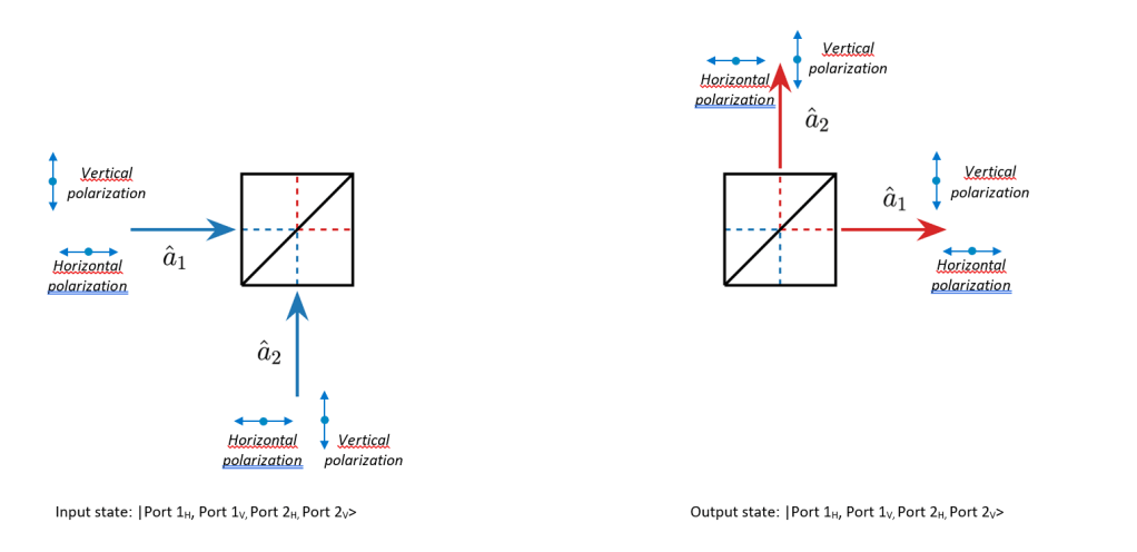
The circuit should have 4 optical channels (two polarizations for the two input ports of the beamsplitter). The channels are:

• Channel 0: Horizontally polarized light at input port a1
• Channel 1: Vertically polarized light at input port a1
• Channel 2: Horizontally polarized light at input port a2
• Channel 3: Vertically polarized light at input port a2

After the beamsplitter the photon number in two channels is measured and written to the two classical channels. We use detectors which are able to determine the photon count in the channels and in this case only measure horizontal polarization.

• The measured photon count in Channel 0 is witten to classical channel 0
• The measured photon count in Channel 2 is written to classical channel 1

This is the Python code to build the circuit

import fock_state_circuit as fsc

circuit = fsc.FockStateCircuit(length_of_fock_state = 3,
                                no_of_optical_channels = 4,
                                no_of_classical_channels=2
                                )

circuit.non_polarizing_50_50_beamsplitter(input_channels_a=(0,1), 
                                          input_channels_b=(2,3)
                                          )

circuit.measure_optical_to_classical(
                 optical_channels_to_be_measured=[0,2],                                   
                 classical_channels_to_be_written=[0,1]
                  )



result = circuit.evaluate_circuit(
             collection_of_states_input=initial_collection_of_states
             )

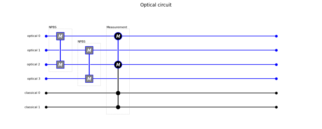
We can draw the schematics of the circuit by calling circuit.draw(). We see that the non-polarizing beamsplitter (NPBS) creates a coupling between channels 0 and 2, and between channels 1 and 3. We also see the measurement node measuring channels 0 and 3 and writing the results to classical channels 0 and 1.

Next we create input states to run through the system. We define an initial_collection_of_states such that the input states are only those where we have one horizontally polarized photon in each input port, or where we have two horizontally polarized photon simultaneously at the two input ports. We describe the optical by a string consisting of the number of photons per channel.

• ‘1000’ means one photon in channel 0 and none in the other channels.
• ‘0010’ means one photon in channel 2 and none in the other channels.
• ‘1010’ means one photon in channel 1, one in channel 2.
• ‘2000’ means two photons in channel 0 and none in the others.

When we call CollectionOfStates(fock_state_circuit=circuit) we create a collection of states set up for the circuit. This collection is loaded with all possible number states. As we are interested in a limited number of states we filter the initial collection.

import collection_of_states as cos

initial_collection_of_states = cos.CollectionOfStates(fock_state_circuit=circuit)

initial_collection_of_states.filter_on_initial_state(
                   initial_state_to_filter=['1000', '0010', '1010']
                   )

Now we can evaluate the circuit for the given input states. We call the function circuit.evaluate_circuit evaluating and get a resulting collection of states back.

result = circuit.evaluate_circuit(
             collection_of_states_input=initial_collection_of_states
             )

result.plot()

The variable results contains the states which result if the input states evolve through the circuit. The resulting states canbe plotted by calling result.plot()

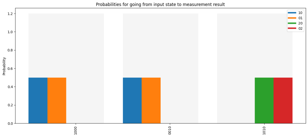
We see in the plot the output histograms for the classical channels (i.e., the measurement results) for the different input states. It is clear that for inputs ‘ 1000’ and ‘ 0010’ (i.e., a horizontally polarized photon in one of the inputs of the beamsplitter) we find the photon with 50% probability in one, and with 50% probability in the other output port. We would expect nothing else for a 50%/50% beamsplitter.

When using two photons we see that only outcomes where we measure 2 photons in channel 0, or 2 photons in channel 2 are seen (each with 50% likelihood). We never see the photons each in a different channel (that would be outcome ’11’ which is not present). Note that the outputs depict the classical channels. We only measure two optical channels so the output only has two digits.

This effect is known as the HOM effect, where photons like to ‘ bunch’ together rather than being separated in different optical channels.

Basic explanation of FockStateCircuits

Circuits

A FockStateCircuit consists of a series of ‘nodes’. The variable circuit.node_list contains the nodes with all relevant information for evaluating the states and displaying the nodes. There are 4 types of nodes:

• Optical nodes: These only contain interactions between optical channels (beamsplitters, wave plates)
• Classical nodes: These only contain interactions between classical channels (e.g., to perform a calculation based on values in these channels)
• Measurement nodes: These contain measurements where classical channels are written with photon numbers measured in the optical channels. The optical channels will ‘collapse’ into the value corresponding to the measurement result
• Combined nodes: These nodes have optical components which characteristics are set by values in the classical channels. This could be a wave plate whose angular orientation and/or phase delay is determined by a value the classical channels.

States

Circuits run collections for states. The collections contain instances of the class `State`. Each state describes pure state which can be run on the circuit (i.e., it has the right number of classical and optical channels). The format for a state is:

Identifier: 'identifier_1-M1a'

Initial state: '10'

Cumulative probability: 1.00

Classical values: ['0.00', '1.00']

Last measurement result:  

    Value: ['0.00', '1.00'], Probability: 1.00

Optical components:

    Component: '01' Amplitude: (1.00 - 0.00i), Probability: 1.00

Below a short description of the different elements of a State:

• initial_state (of type string) : Typically the state from which the current state has evolved in the circuit, but users can customize for other purposes. Also used to group together states in a statistical mixture. In that case each state in the mixture needs to have the same ‘ initial_state’ and the ‘ cumulative_probabilities’ (see next) need to add up to 1.
• cumulative_probability (of type float) : Probability to evolve from initial state to current state (as consequence of measurement or decoherence). Alternatively used to give the weight of this state in a statistical mixture of states indicated with the same initial_state.
• optical_components (of type dictionary) : These are the optical components of the state described as number states per channel (i.e., ‘1001’ means one photon in channel 0 and channel 3). Each component has an amplitude (complex number) and a probability (float). The probability is always the square of the absolute value of the amplitude (so effectively redundant information, but nice to have). The format for optical_components is like in this example where components ‘ 1011’ and ‘ 1110’ are in a superposition with equal amplitudes: { '1011': {'amplitude': 0.71 + 0j, 'probability': 0.5}, '1110': {'amplitude': 0.71 + 0j, 'probability': 0.5}}
• classical_channel_values (of type list): A list holding the values for classical channels in the fock state circuit.
• measurement_results (of type list of dictionaries) : Measurement_results holds the outcomes of all measurements. New measurements should appended to the end of the list.At each measurement the classical channel values after the measurement are store together with the probability to get that measurement result. The format for measurement results is as in this example: [{'measurement_results': [1, 3, 3.14], 'probability': 0.5}, {'measurement_results': [0, 0, 3.14], 'probability': 0.25}]

Watch outs

When defining a circuit the parameter length_of_fock_state has to be set. If length_of_fock_state is for instance 3 the possible values for any optical channel are 0, 1 or 2 photons. So the maximum photon number in this case is 2. In general the maximum photon number is equal to (length_of_fock_state-1). When the system encounters a transition between Fock States where the photon number is larger than (length_of_fock_state-1) it will artificially set the transition amplitude to 1, leading to non-physical outcomes.

After measurement the optical states ‘collapses’ to the value corresponding to the measurement. If more measurement outcomes are possible one state will turn into a statistical mixture. Note that the photons will not disappear once they are measured (so this is a kind of ‘non-destructive measurement’. We do get collapse of the wave function but photons are not absorbed in the detection process).

Under the hood the system uses quite large data structures. The basis is typically of size length_of_fock_state to the power no_of_optical_channels. There is some optimization to reduce the size of these matrices but it is still wise to minimize values to lowest number possible. This is also the reason to cap the number of photons by setting length_of_fock_state to the right value for the system

Documentation

On github you will find more information as well as the source code. We are working on making the package available on PyPi, but right now GitHub is the only source. Next to the source code (in directory ‘ src‘ ) you als find a tutorial and the pydoc documention in directory ‘ docs‘ .