The armchair quantum physicist

Introduction

Entanglement and the related ‘instantaneous’ influence over a distance is one of the most intriguing phenomena modern physics, maybe even in modern science. The 2023 Nobel prize has been awarded for progress made in this domain. The storyline starts with the 1935 paper by Einstein, Podolsky and Rosen stating that quantum theory is so counter-intuitive that it must be wrong. Major milestones are formulation of Bell’s inequalities in 1964 and the 1982 experiment by Alain Aspect demonstrating that quantum theory is right, and our intuition is wrong. Until this day the scientific debate continues with respect to the interpretation of quantum physics. In parallel applications of the most fundamental concepts in quantum computing are rapidly developing, not hindered by open questions on interpretation.

In a previous post we simulated Alain Aspect’s experiment using Python Qutip and provided a coin game as analog to the experiment. In this post we dive deeper into the paradox and try to use simple coin games to bring across the strangeness of quantum theory. We then continue to  show how we can easily simulate the experiment using Python FockStateCircuit. It is exciting that what was a gedankenexperiment in 1935 and a major achievement in experimental physics in 1982 is by now something which can be demonstrated by using some simple code.

Reference articles

1. Einstein, A.; Podolsky, B.; Rosen, N. (1935). “Can Quantum-Mechanical Description of Physical Reality Be Considered Complete?”. Physical Review 47 (10): 777–780
2. Bell, J.S. (1965). “On the Einstein Podolsky Rosen paradox”. Physics Physique Fizika 1, 195
3. Clauser, J. F.; Horne, M.A.; Shimony, A.; Holt, R.A. (1969). “Proposed Experiment to Test Local Hidden-Variable Theories”. Physical Review Letters. 23 (15): 880–884.
4. Clauser, J.F.; Horne, M.A.  (1974). “Experimental consequences of objective local theories”. Phys. Rev. D. 10 (2): 526–35.
5. Aspect, A.; Grangier, P.; Roger, G. (1981). “Experimental Tests of Realistic Local Theories via Bell’s Theorem” Phys. Rev. Lett. 47 (7): 460-3.
6. Aspect, A.; Grangier, P.; Roger, G. (1982). “Experimental Realization of Einstein-Podolsky-Rosen-Bohm Gedankenexperiment: A New Violation of Bell’s Inequalities”. Phys. Rev. Lett. 49 (2): 91–4.
7. Aspect, A.; Dalibard, J.; Roger, G. (1982). “Experimental Test of Bell’s Inequalities Using Time-Varying Analyzers”. Physical Review Letters. 49 (25): 1804–7
8. Hensen, B.; Bernien; H.; Dréau, A. et al. “Loophole-free Bell inequality violation using electron spins separated by 1.3 kilometres”. Nature 526, 682–686 (2015).

The Einstein, Podolsky and Rosen paper from 1935

Einstein, A.; Podolsky, B.; Rosen, N. (1935). “Can Quantum-Mechanical Description of Physical Reality Be Considered Complete?”. Physical Review 47 (10): 777–780

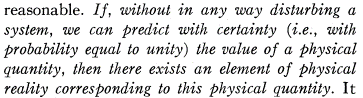
The discussion on an experiment to (dis)proof the completeness of quantum theory starts with the famous article by Einstein, Podolsky and Rosen in 1935. This article states that ‘it is generally assumed that the wave function does contain a complete description of the physical reality of the system’. The authors define reality as our ability to predict the outcome of a measurement:

We already know that if two operators are non-commuting (like position and momentum of a particle) we cannot measure both with arbitrary precision. If we for instance know the momentum of a particle to be exactly , we cannot predict its position.

We intuitively know that both momentum and position for a particle are real, even if we cannot measure them both. From this argument EPR conclude that there must be something missing in quantum theory: “Clearly quantum theory does not provide a complete description of physical reality, but maybe another description exists that would provide this complete description”.

John Bell in 1964

Bell, J.S. (1965). “On the Einstein Podolsky Rosen paradox”. Physics Physique Fizika 1, 195

Now we fast forward in time to 1964, when John Bell presents his article. He demonstrates that if we assume there is any variable or set of variables describing physical reality completely this would lead to an upper bound for certain correlations between independent measurements. This sounds quite abstract, so let’s try to make it tangible. Below we analyze the original reasoning from Bell and apply it to a game of coins to define the upper bound to possible correlations.

John Bell considers a system where two particles are generated and travel in different directions. The particles are in a ‘singlet spin state’, which means we do not know the spin of any individual particle, but we know that their total spin is zero. If the particles are photons we know that they always have orthogonal polarization although for every individual photon the polarization will appear random. Bell continues to describe detection of one particle in polarization direction ‘a’, and the second in polarization direction ‘b’ or ‘c’. Any of these detections will yield outcome +1 (if the polarization is parallel with the detector), or -1 (if the polarization is detected as orthogonal).

Intermezzo: There can be a lot of confusion around some conventions. Within this blogpost we try to be consistent and for that reason can deviate from the original publication. Two main sources of confusion are:

1. In this post we use photons. This is in line with the experiments by Alain Aspect. Originally John Bell considered electrons. Between angles for detecting electron spins and for photons polarization there is a factor of 2: Two electrons have opposite spin if the angle between the spin directions is 180 degrees (up or down), two photons have opposite polarization if the angle is 90 degrees (horizontal or vertical).
2. In this blogpost we use ‘+1’  for maximum correlation, i.e., for the situation where two photons have the same polarization. If the correlation is ‘-1’ they always have orthogonal polarization. John Bell adds a minus sign to his definition of correlation because in the singlet state the electrons have opposite spin. This difference leads to a minus sign in our ‘Bell inequality’ as compared to what is originally published by John Bell.

Let’s first simulate the ‘gedankenexperiment’ of John Bell with coins. We have a ‘dealer’  and two players. The dealer gives one player a 2 euro coin, and the other played a 2 euro coin and a 1 euro coin. At random the decision is taken (after the dealer handed out the coins, without anyone knowing how the dealer placed the coins) which two coins will be evaluated in this turn (so either both 2 euro coins, the 2 euro from the first player and the 1 euro coin from player two, or both coins from player two). With this setup of the coin game, we mimic the experiment John Bell has in mind. The two coins for player 2 represent one particle where two possible measurements can be done.

For every turn the players note down a ‘+1’ if they detect ‘head’ and ‘-1’ if they detect ‘tail’. We call the result noted by the first player (on his 2 euro coin) ‘a’. We call the result noted by the second player ‘b’ for his 2 euro coin and ‘c’ for his 1 euro coin. After playing the game for a certain number of turns the results are put together in a table like this one:

Turn	First player	Second player
	a (two euro coin)	b (two euro coin)	c (one euro coin)
1	1	1
2	-1	-1
3	1		1
4		-1	-1
5	-1		1
6		1	-1
7	1		-1
8	1	-1

First, we should note that if played correctly the average value of the numbers in columns ‘a’,’b’ and ‘c’ should be zero (we had for any coin as many observation of ‘head’ as for ‘tail’). We can also look at correlation and note for every turn the product of the numbers in for instance columns ‘a’ and ‘b’. If the average of this value is also zero the dealer did not create any correlation between the two euro coins given to layers 1 and 2 (we call this no correlation). If the average value of this product would be ‘1’ we know that the dealer for the two euro coin always gave both players the same value. Either both received head, or both received tail (this we would call perfect correlation). If the average value of the product would be -1 we know the dealer always gave one player a two euro coin heads up, and the other player a two euro coin tails up (perfect anti-correlation)

John Bell evaluates the average value of the products ‘ab’, ‘ac’ and ‘bc’. In our table we can add some columns to note down for each turn the result for the applicable product. The averages are then the average values in columns ‘ab’, ‘ac’ and ‘bc’

Turn	First player	Second player		Evaluation of ‘products’ after the game
	a	b	c	ab	ac	bc
1	1	1		1
2	-1	-1		1
3	1		1		1
4		-1	-1			1
5	-1		1		-1
6		1	-1			-1
7	1		-1		-1
8	1	-1		-1

Now for the coins the fundamental assumption is that even the coins we did not evaluate in a turn still have a value. These coins are really there, and they really are positioned ‘heads up’ or ‘tails up’. Whether we look at them does not matter as we belief there is a reality independent of our observation. If we take this assumption, we can determine some limits to the possible outcomes of the game. For instance. If  is equal to ‘1’ we know b and c always are equal. We then know that ab – ac is always zero, so . On the other hand,  if would be -1 we know that b and c would always be opposite, so is either 2 or -2. From this we can derive that

This is the inequality as presented by Bell in his 1964 paper (except for a minus sign he includes in his derivation, for John Bell the average   would be -1 while we took this as 1).

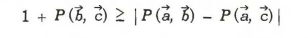
This inequality holds if we assume that when we measure a +1 or -1 measure for a, b and c are this is as ‘real’ as when we measure a coin to heads up or tails up. The fundamental aspect is that a real value is there even if we do not measure it.

John Bell evaluated his inequality for two spin ½ particles in a singlet state. We take an entangled photon pair for this. If for instance the photons are in state we should find both photons in identical polarization. Imaging we take for ‘a’ the horizontal direction, for ‘b’ detection at an angle of 45 degrees and for ‘c’ detection at 22.5 degree. We then know that should be 0. and should be . So the equality then is , or 0.71 < 0.29. This is clearly incorrect so the quantum prediction violates the bell inequality. Where Einstein Podolsky and Rosen posed their paradox to proof that quantum theory gives inconsistent results, the experiment proposed by Bell would indicate that quantum theory is right and our intuitive assumptions around physical reality are wrong!

The CSHS inequality

Clauser, J. F.; Horne, M.A.; Shimony, A.; Holt, R.A. (1969). “Proposed Experiment to Test Local Hidden-Variable Theories”. Physical Review Letters. 23 (15): 880–884.

Clauser, J.F.; Horne, M.A.  (1974). “Experimental consequences of objective local theories”. Phys. Rev. D. 10 (2): 526–35.

After the 1964 paper by John Bell multiple versions of the Bell inequalities were proposed. The reason for this diversity was the ambition to generate experimental proof with sufficient accuracy. Practical considerations like detector efficiencies and the fact that particles are destroyed in measurement had to be considered. Let us dive deeper into two versions.

In 1969  John Clauser, Michael Horne, Abner Shimony, and Richard Holt (CHSH) proposed a “generalization of Bell’s theorem which applies to realizable experiments”. The 1974 paper by John Clauser and Michael Horne in the appendix develops a different formulation for Bell’s inequality nowadays often referred to as the CHSH inequality. It is this CSHS form of the Bell inequality that is experimentally demonstrated by Alain Aspect in his July 1982 paper.

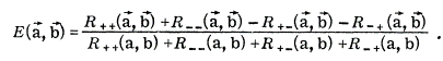
To explain the CSHS inequality we start with the schematics of the measurement set-up used by Alain Aspect in his July 1982 paper.

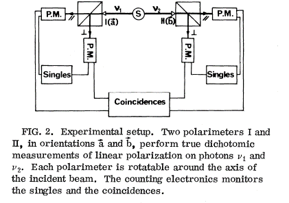
This setup has a source emitting two particles (photons), one photon to detector 1 and the other to detector 2. The detectors determine whether the photon is polarized in a certain direction or orthogonal to this direction. For detector 1 this direction is called ‘a’, and for detector 2 this direction is called ‘b’. If the photon polarization is detected parallel to ‘a’ we note the result as +1, if the polarization is orthogonal to direction ‘a’ we note as result -1 (and the same for detection parallel or orthogonal to ‘b’ for the other detector). The setup is built such that the detection direction can be rotated by physically rotating the detectors. In this we can measure polarization in any direction. Specifically for the experiment we use two directions for each detector, which we call a or a’ for detector 1 and  b or b’ for detector 2.

The fact the photon is detected in both polarization directions rather than being absorbed in a polarizer makes the data processing a lot easier (when using absorbing polarizers, you never know whether the photon was not there in the first place, whether it was absorbed or whether the detector failed to detect). The setup with 4 detector and  polarization beamsplitters allows for positive identification after a click of any two detectors.

So in the experiment for every run we set the detector 1 to a or a’ and detector 2 to direction b of b’. We then measure polarization parallel or orthogonal and note down a +1 or -1 for both detectors. From this we can determine the correlations , , or as the average value of the products of detection result for detectors 1 and 2. The CSHS inequality then states that:

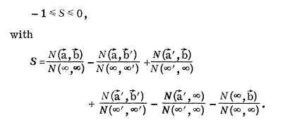
To use the CSHS inequality in the form stated above we need to measure the two orthogonal polarization direction for the photons (or the two opposite spin directions for electrons). In some set-ups this is not possible. We can re-formulate the inequality to deal with the situation where we only detect one polarization or spin direction for each particle. For completeness let’s also mention a different version of the same inequality which can be derived from the above.

Consider the value is the correlation between measurements a and b, but is also the average of the product ab over all runs of the experiment.

Here is the probability to find result ‘1’ for both measurement ‘a’ and measurement ‘b’. If we take measurement ‘a’ to be independent of measurement ‘b’ we can factor out these probabilities

If we then consider that we always measure a particle as either ‘+1’ or ‘-1’ we find:

And with this we rewrite the CSHS inequality as

This is often referred to as the CH74 inequality. Note that in this derivation we had to ‘factor’ the probabilities for a combined outcome for both particles into the probabilities for individual particles: . This factoring already assumes a form of locality.

Intermezzo: There can be confusion on the ‘name’ used to distinguish the various forms of the Bell inequality. The original inequality mentioned in Bell’s 1965 paper is quite clear, although the paper is also sometimes referred to as the 1964 paper. The abbreviation CHSH stands for John Clauser, Michael Horne, Abner Shimony, and Richard Holt who jointly published their paper in 1969. The exact form seen nowadays does however only show in the 1974 paper by John Clauser and Michael Horne. Interestingly, in the 1974 paper John Clauser and Richard Horne state that this form of the inequality comes from John Bell himself although not explicitly mentioned. (“Bell does not write Eqs. (B1), but this definition is implicit in his discussion.”). So whether the CSHS inequality now originates from Clauser, Horne, Shimony, and Holt, from John Bell or was first noted down by Clauser and Horne cannot be traced back from formal literature. Also in exact form we see both the CSHS inequality and the CH74 inequality both for the first time in the 1974 paper.

Understanding the CHSH inequality

Just as we assessed the original Bell inequality by applying it to a coin game we also assess the CSHS inequality. The experiment we want to keep in mind is where we have a pair of particles, each send to a separate detector. Each detector has two possible settings (a or a’ for one detector and b or b’ for the other). So in total there are four possible settings for the detectors (ab, ab’, a’b or a’b’). Each measurement gives an outcome of either ‘+1’or ‘-1’. For pair of measurements we determine the correlation. This correlation is a number between 1 (perfect correlation) and -1 (anti-correlation). If the correlation between ‘a’ and ‘b’ is 0 we are as likely to measure ‘1’ or ‘-1’ for b after we measure ‘1’ for a. If the correlation is -1 we will always measure ‘-1’ for b after we measure ‘1’ for a, and will always find ‘1’ for b if we find ‘-1’ for a.

In formulas, the correlation is the average value of the product ‘ab’ over all measurements. So if you have 10 turns then for each turn you determine the value for ‘ab’, and the correlation (noted as <ab> is the average value for this product:

We can express the same in probabilities. If the probability of find a ‘1’ for both a and b is expressed as then the average value for <ab> is:

When ‘a’ and ‘b’ are equal the value for ‘ab’ is 1, if they are different the value is -1. So we can also define the probability to get an equal outcome , and similarly the probability to get and unequal outcome . We then see:

(In the second line we used the fact that the outcomes are either equal or unequal, so and must add up to 1).

We have defined some simple rules for the correlation between measurement outcomes at detectors ‘a’ and ‘b’. Of course these same rules hold for the correlation between a’ and b, a and b’, a’ and b’ (where we put the ‘ is arbitrary and should not define the outcome).

Now we want to derive the Bell inequalities and show that with simple assumptions there is an upper and lower limit to some combined correlations. We can for instance look at (ab + ab’ + bb’).

At first sight we could think that the value for is bound between -3 and 3 because any of the terms is bound between -1 and 1. Closer inspection shows that the range is smaller. For every individual turn either b_i=b_i’ (and b_ib_i’ = 1) or b_i=-b_i’ (and b_ib_i’ = -1). In the first case either ab = ab’ = 1, or ab = ab’ = -1. In the second case either ab = 1 and ab’ = -1, or ab = -1 and ab = 1. In any case the possible outcomes for the total ab + ab’ + bb’ is larger than -1. The outcome -3 never occurs as it would require b to be different from b’, and a to be different from b and b’ at the same time. But if we know that b and b’ are different we know that a has to equal to at least one of them. So we logically derive:

Now look at <ab – ab’ – bb’>. Either the b’s are equal  (b=b’, bb’  = 1), then (ab – ab’ – bb’) is always -1. If on the other hand b is not equal to b’ (bb’  = -1) then either ab = 1, ab’=-1 or ab = -1, ab’ = +1. So we never find a value for (ab – ab’ – bb’) lower than -1 (it would require b and b’ to be equal, but at the same time a to be unequal to b and a to be equal to b’). This reasoning would also hold if we evaluate <a’b – a’b’ – bb’>, so we know:

If  we now add up the inequalities we can establish a lower bound for a combination of detector settings at both sides.

Now let’s try to find an upper bound as well. Look at ab + ab’ – bb’. If b=-b’ this value is always +1, if b = b’ either ab = -1 and ab’=-1 or ab = 1 and ab’=1. So total is -3 or 1. So we know for sure that the possible outcomes for the total ab + ab’ – bb’ are smaller than +1

And also we can evaluate -ab + ab’ + bb’

And as we know the result should hold equally for a’ and for a we also know:

Combining these

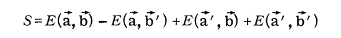
So we have established the CHSH inequality

The Alain Aspect experiments from 1982

Aspect, A.; Grangier, P.; Roger, G. (1981). “Experimental Tests of Realistic Local Theories via Bell’s Theorem” Phys. Rev. Lett. 47 (7): 460-3.

Aspect, A.; Grangier, P.; Roger, G. (1982). “Experimental Realization of Einstein-Podolsky-Rosen-Bohm Gedankenexperiment: A New Violation of Bell’s Inequalities”. Phys. Rev. Lett. 49 (2): 91–4.

Aspect, A.; Dalibard, J.; Roger, G. (1982). “Experimental Test of Bell’s Inequalities Using Time-Varying Analyzers”. Physical Review Letters. 49 (25): 1804–7

Hensen, B.; Bernien; H.; Dréau, A. et al. “Loophole-free Bell inequality violation using electron spins separated by 1.3 kilometres”. Nature 526, 682–686 (2015).

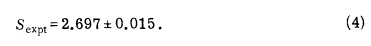
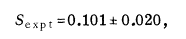
Alain Aspect together with his co-workers from the “Institut d’Optique Theorique et Appliquee, Universite Paris-Sud” published three articles in a very short timeframe demonstrating experimental confirmation of the violation of Bell’s inequality. In the first and second article they used the single-channel version of the CHSH inequality (aka CH74) and in the second article they used the CHSH formulation of the equality. All set-ups used entangled photons with polarization sensitive detection.

From the 1981 article we see the CH74 formulation was used.

From the article July 1982 we see the CHSH formulation was used

From the December 1982 paper we see

These experiments by the French grouped triggered a development towards true loophole free confirmation of the Bell inequality violation. It was not until over 30 years later that the first claim to this loop-hole free experiment was made by the QuTech group at Delft University of Technology in The Netherlands. They used electron spin in an experiment where no further assumption was required to interpret the results. Their value for S in the CHSH formulation was S = 2.42 +/- 0.2.

Demonstrating violation of Bell’s inequality in Python

In the tutorial for ‘FockStateCircuit’ (see GitHub) the experiment of Alain Aspect is simulated.

We have a source of entangled photons which travel in two different directions. Then we have detectors behind polarizers oriented at different angles. We are interested in determining the correlation between detecting a photon in at one side and detecting a photon at the other side for different angles of the polarizers. For each side we have two settings for the polarizer: a and a’ at one side and b and b’ at the other side.

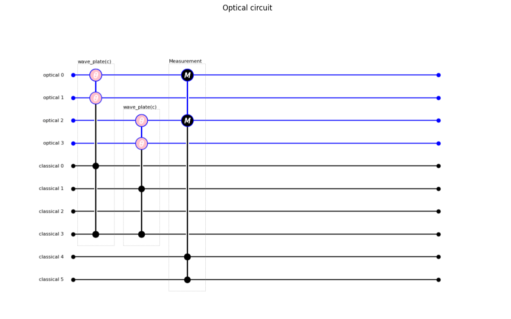
We will model this by using a FockStateCircuit with  4 channels. Channel 0 and 1 represent the system to the left of the photon generation and channel 2 and channel 3 represent the system to the right. We then use detecors in channel 0 and channel 2 representing the detection in a polarization direction in which photons are detected and channels 1 and 3 to represent the orthogonal polarization. A half-wave plate in front of the detector determines the exact polarization angle which is detected. Below the schematics of the FockStateCircuit are generated by the command circuit.draw()

The polarization angles for which we expect maximum violation of the Bell inequality is

*

*

*

*

We run the circuit for these for settings by iterating through the dictionary polarization_settings

polarization_settings = {'ab' : {'left': 0  , 'right' : math.pi/16},

                       'a\'b': {'left': 0 , 'right' : 3*math.pi/16},

                        'ab\'' : {'left': math.pi/8 , 'right' : math.pi/16},

                        'a\'b\'' : {'left': math.pi/8 , 'right' : 3*math.pi/16 }}

As input we use an entangled state such that either both photons are horizontally, or both photons are vertically polarized

entangled_state.optical_components = {
     '1010' : {'amplitude': math.sqrt(1/2), 'probability': 0.5},
     '0101' : {'amplitude': math.sqrt(1/2), 'probability': 0.5}
     }

For each of the polarization setting we measure the correlation as . The higher the likelihood for the same outcome left and right, the higher this correlation. The parameter is then defined as . Classical theory limits this to values between -2 and 2. The prediction from quantum theory is that is for the specific angles mentioned above.

If we run our system with the `entangled_state`  as input and the half-wave plate orientation angles defined in `polarization_settings` we find exactly the value we expect from quantum mechanics:

S for entangled state and polarization settings for maximum Bell inequality violation:  2.8284267323312253

The code to generate this result is

import fock_state_circuit as fsc
import collection_of_states as cos
import imp
import math
import numpy as np
%matplotlib inline
import matplotlib.pyplot as plt

circuit = fsc.FockStateCircuit(length_of_fock_state = 2, 
                                no_of_optical_channels = 4,
                                no_of_classical_channels=6)

# orient polatizers before detectors
circuit.wave_plate_classical_control(optical_channel_horizontal=0,
                                     optical_channel_vertical=1,
                                     classical_channel_for_orientation=0,
                                     classical_channel_for_phase_shift=3)
circuit.wave_plate_classical_control(optical_channel_horizontal=2,
                                     optical_channel_vertical=3,
                                     classical_channel_for_orientation=1,
                                     classical_channel_for_phase_shift=3)

circuit.measure_optical_to_classical(optical_channels_to_be_measured=[0,2],classical_channels_to_be_written=[4,5])
circuit.draw()

# define the angles we need for the half-wave plates in order to rotate polarization over the correct angle
polarization_settings = {'ab' : {'left': 0  , 'right' : math.pi/16},
                        'a\'b': {'left': 0 , 'right' : 3*math.pi/16}, 
                        'ab\'' : {'left': math.pi/8 , 'right' : math.pi/16}, 
                        'a\'b\'' : {'left': math.pi/8 , 'right' : 3*math.pi/16 }}

# First create an entangles state where both photons are either both 'H' polarized or both 'V' polarized
# The optical state is 1/sqrt(2)  ( |HH> + |VV> )

initial_collection_of_states = cos.CollectionOfStates(fock_state_circuit=circuit)
entangled_state = initial_collection_of_states.get_state(initial_state='0000').copy()
initial_collection_of_states.clear()
entangled_state.initial_state = 'entangled_state'
entangled_state.optical_components = {'1010' : {'amplitude': math.sqrt(1/2), 'probability': 0.5}, '0101' : {'amplitude': math.sqrt(1/2), 'probability': 0.5}}


S_ent = []
E = []

for key, setting in polarization_settings.items():
    initial_collection_of_states.clear()
    state = entangled_state.copy()
    state.classical_channel_values = [setting['left'],setting['right'], 0, math.pi,0,0]
    state.initial_state = 'entangled_state_' + key
    state.cumulative_probability = 1
    initial_collection_of_states.add_state(state)
    result = circuit.evaluate_circuit(collection_of_states_input=initial_collection_of_states)
    result11 = result.copy()
    result11.filter_on_classical_channel(classical_channel_numbers=[4,5], values_to_filter=[1,1])
    probability11 = sum([state.cumulative_probability for state in result11])
    result00 = result.copy()
    result00.filter_on_classical_channel(classical_channel_numbers=[4,5], values_to_filter=[0,0])
    probability00 = sum([state.cumulative_probability for state in result00])
    E.append(2*(probability00+probability11)-1)
    
S_ent = E[0] - E[1] + E[2] + E[3]

print("S for entangled state and polarization settings for maximum Bell inequality violation: ", S_ent)