
In previous posts, we addressed the challenge posted by Einstein on quantum theory in the 1930s [1], the response from John Bell in the 1960s [2], and the experimental evidence in favor of quantum mechanics provided by Alain Aspect in the 1980s [3]. In this post, we evaluate what aspects of quantum physics are challenged by Einstein and how these come back in the experiments. This also shows how quantum mechanics deviates from our intuitive everyday worldview.
We use a generic (though)experiment that consists of two particles and two observers (at different locations) receiving one particle. The observers can choose to perform a measurement T or a measurement S on their particle. The outcomes of the measurement are either ‘1’ or ‘-1’, and for any individual observer, the result will appear totally random. We then evaluate the correlation between the results for the observers. So, after repeating the experiment, we look for the average value of the result for SS (if both observers decided to measure the quantity S), ST, TS, and TT. The Bell inequality states that:
-2 ≤ <SS> + <ST> + <TS> — <TT> ≤ 2
Here, the symbol <> denotes the average value: < SS> is the average value obtained over a large number of repetitions where both observers select measurement S. If they always measure the same outcome, this average is 1; if they always measure opposite outcomes the average is -1, and if their outcomes are uncorrelated, the average will be 0.
Commutating observables and EPR
In a coin game, we used a cup covering two coins (a Two euro coin and a Single euro coin) as a ‘particle.’ The players in the game (the observers) each receive one cup with two coins. They can choose to select the S or the T coin to measure whether it is heads up or tails up. The payout for this game is one cent per turn when both players select coins in the same orientation, except when they both select the T coin. In that case, they win when their coins have opposite orientations. They have to pay one cent if they do not win in a turn. So, for each turn, their payout is either + 1 cent or -1 cent. For this game, we can prove that the payout over many turns has to be between -0.5 cents and + 0.5 cents (boundary values included). This is the CHSH limit, a variant of Bell’s inequalities.
When we derive the upper bound to the CHSH correlation for this game, we use the fact that the S coin still has a defined value even if a player selects the T coin. All four coins have a well-defined value for each turn: for any coin in a given turn, we can say it is heads up or tails up. Maybe the players do not know the orientation if the coin is covered, but the value is ‘real.’
In his experiment, Alain Aspect uses photons rather than coins. For each photon, he chooses to measure horizontal polarization T or diagonal polarization S. If we would like to use the same argument we used in the coin game and assign a value to the diagonal polarization when we measure horizontal, we run into an issue. The two observables are non-commuting, and we cannot speak about the hypothetical outcome of the S measurement when we have measured T. If two quantities are non-commuting, they share an uncertainty relationship in quantum mechanics. If we measure one of these quantities with high accuracy, we have to accept that we have a high uncertainty for the value of the other quantity. Heisenberg introduced this fundamental concept in quantum physics in 1927.
So, the logic leading to the upper bound on the CHSH correlation needs to be revised for quantum mechanics when we select non-commuting observables. Einstein stated in the introduction of his 1935 paper [1]:
“In quantum mechanics, in the case of two physical quantities described by non-commuting operators, the knowledge of one precludes the knowledge of the other. Then either (1) the description of reality (…) is not complete or (2) these two quantities cannot have simultaneous reality.”
Einstein argued that (2) cannot be correct and, therefore, (1) has to be the case. Since we now observe a violation of Bell’s inequality, we have to accept that (2) can be the case and that due to quantum mechanics, our notion of ‘reality’ has to be adjusted.
The concept of observable quantities that do not commute is fundamental to the EPR paradox and the Bell inequality. In fact, with simple math, it can be shown if T and S commute, the value of the CHSH inequality is bound between 2 and -2, even if the two particles are in an entangled state. So, non-commuting observables are a condition for violation of Bell’s inequality.
Entanglement, tensor product, and conditional probability
We concluded in the previous paragraph that non-commuting observables are necessary to break the CHSH inequality. However, this condition by itself is not enough. The second quantum mechanical concept we need is entanglement.
In the experiment, the two observers get ‘random’ results for their photon (or for their coin). By looking at their data, they cannot conclude anything on the measurement performed by the other observer. However, to violate Bell’s inequality, we must allow the measurement result for one particle to alter the probability distribution for the other particle. If a detector clicks on one side of the setup, the probability of detecting the particle on the other side is instantaneously changed. Quantum mechanics does describe this instantaneous effect but does not provide any interaction mechanism that explains how the probability distribution in one place is affected by the measurement outcome in another place. As Einstein stated [1]:
“We see therefore that, as consequence of two different measurements performed upon the first system, the second system may be left in states with two different wave functions. On the other hand, since (..) the two systems no longer interact, no real change can take place in the second system in consequence of anything that may be done to the first system.”
When Bell’s inequality is violated, the information contained at the location for the second photon is altered or augmented based on the measurement outcome for the first particle. In quantum mechanics, the wavefunction describes the state of a system. Generally, this wavefunction splits into a part for the first particle and a part for the second particle. The wavefunction for the complete system is then the product of the wavefunctions for the separate particles. In that case, the wavefunction describes the state of the first particle ‘in isolation’ and the state of the second particle ‘in isolation .’ When the particles are entangled, this split is impossible (in fact, this is the definition of entanglement: we cannot write the wavefunction for the complete system as a product of the wavefunctions for the separate sub-systems). In this entangled case, quantum mechanics describes that based on measurement for one particle, the wavefunction globally and instantaneously ‘collapses’ to match the measurement result. This collapse changes the second particle’s probability distribution, enabling correlations that violate Bell’s inequalities.
We have to accept that there are non-local aspects to quantum theory. It is the case that the probability of finding a particular measurement outcome (and therefore the locally present wave function) can be instantaneously affected based on distant events.
Entanglement is a necessary condition for violating Bell’s inequality. Entanglement occurs when we cannot ‘split’ the wavefunction into a part for the first particle and a part for the second particle. For this reason, in an entangled state, we cannot define the state of the first particle in isolation. We cannot make any statement on the polarization of this first particle. It is not that we do not know this polarization; it is fundamentally ‘unknowable .’ For this reason, any polarization measurement on the first particle will give a random result. This randomness for an individual particle is fundamental to entanglement and, therefore, to violating Bell’s inequality.
In popular science, a few quotes from Einstein regularly appear. His question to Abraham Pais: “Is the moon really there if we do not look at it?” [3], his comment on entanglement, “spooky action at a distance” [4], and his objection to the probabilistic nature of quantum mechanics, “I am convinced that does not throw dice” [5]. These statements all come together in the EPR paradox where the concept of non-commuting observables challenges reality, entanglement leads to spooky non-locality, and randomness is a necessary aspect of entangled states.
Where does this bring us?
In this post, we asked ourselves what created the possibility that photons break the limits of the CHSH correlation/Bell inequality. What aspect of quantum mechanics triggers the deviation from classical, intuitive behavior?
- One answer is that the measurements of different polarization directions can be non-commuting for photons. If we measured commutating observables, we would not see any correlation violating Bell’s inequality.
- The second answer is in the entanglement, where we cannot separate the wavefunction in a part of the first photon and a part of the second photon. We can only describe the wavefunction for the combined system of both photons. This means that any measurement result on one photon will affect the probability distribution for a measurement on the second photon.
Both of these conditions need to be in place for a violation of Bell’s inequalities. If we take entangled photons and select measurements T and S in the horizontal and vertical direction (so T and S as orthogonal polarization measurements perfectly commute), the CHSH value would be between 2 and -2. For non-entangled photons, we only see correlation within the bounds of Bell’s inequality, even if we would measure T and S in horizontal and diagonal directions. The combination of the quantum concept which challenges reality, and the quantum concept which challenges locality, leads to the correlations refuted by Einstein but observed by Alain Aspect.
In the next post, we get more mathematical and use vectors and 2×2 matrices to show how polarization measurements on entangled photons can break Bell’s inequalities. We will also see that within quantum mechanics, there is an upper limit to this CHSH correlation. So not only do we have a CHSH value marking the boundary between a classical and a quantum domain, but also a CHSH value marking the boundary between the quantum domain and potentially a super-quantum domain. In the meantime, please leave your comments and builds.
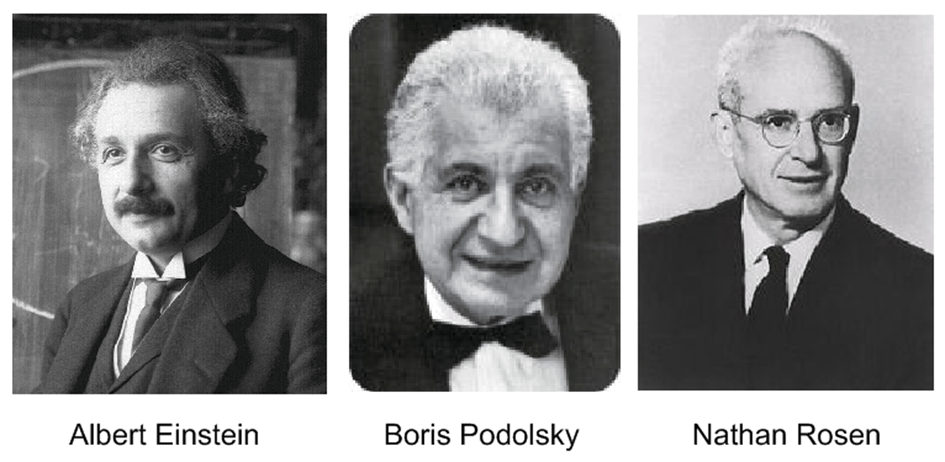
[1] A. Einstein, B. Podolsky, and N. Rosen, “can quantum-mechanical description of physical reality be considered complete?” Phys. Rev. 47, 777 (1935).
[2] JS Bell, “On the Einstein Podolsky Rosen paradox,” Physics 1, 195 (1964).
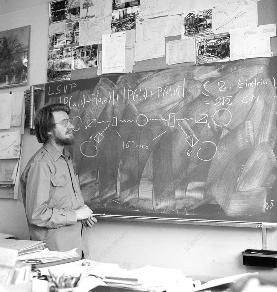
[3] A. Aspect, P. Grangier, and G. Roger, “Experimental Realization of Einstein-Podolsky-Rosen-Bohm Gedankenexperiment: A New Violation of Bell’s Inequalities,” Phys. Rev. Lett. 49, 91 (1982).
[4] “I am at all events convinced that He does not play dice,” The Born-Einstein Letters, with comments by M.Born, Walker, New York (1971).
[5] “We often discussed his notions on objective reality. I recall that during one walk Einstein suddenly stopped, turned to me and asked whether I really believed that the moon exists only when I look at it.” A.Pais, Rev. Mod. Phys. 51, 863 (1979).
[6] “I cannot seriously believe in the quantum theory because it cannot be reconciled with the idea that physics should represent a reality in time and space, free from spooky actions at a distance.” The Born-Einstein Letters, with comments by M.Born, Walker, New York (1971).
EPR, Bell’s inequalities, and Alain Aspect’s experiments
In previous posts, we addressed the challenge posted by Einstein on quantum theory in the 1930s [1], the response from John Bell in the 1960s [2], and the experimental evidence in favor of quantum mechanics provided by Alain Aspect in the 1980s [3]. In this post, we evaluate what aspects of quantum physics are challenged by Einstein and how these come back in the experiments. This also shows how quantum mechanics deviates from our intuitive everyday worldview.
We use a generic (though)experiment that consists of two particles and two observers (at different locations) receiving one particle. The observers can choose to perform a measurement T or a measurement S on their particle. The outcomes of the measurement are either ‘1’ or ‘-1’, and for any individual observer, the result will appear totally random. We then evaluate the correlation between the results for the observers. So, after repeating the experiment, we look for the average value of the result for SS (if both observers decided to measure the quantity S), ST, TS, and TT. The Bell inequality states that:
-2 ≤ <SS> + <ST> + <TS> — <TT> ≤ 2
Here, the symbol <> denotes the average value: < SS> is the average value obtained over a large number of repetitions where both observers select measurement S. If they always measure the same outcome, this average is 1; if they always measure opposite outcomes the average is -1, and if their outcomes are uncorrelated, the average will be 0.
Commutating observables and EPR
In a coin game, we used a cup covering two coins (a Two euro coin and a Single euro coin) as a ‘particle.’ The players in the game (the observers) each receive one cup with two coins. They can choose to select the S or the T coin to measure whether it is heads up or tails up. The payout for this game is one cent per turn when both players select coins in the same orientation, except when they both select the T coin. In that case, they win when their coins have opposite orientations. They have to pay one cent if they do not win in a turn. So, for each turn, their payout is either + 1 cent or -1 cent. For this game, we can prove that the payout over many turns has to be between -0.5 cents and + 0.5 cents (boundary values included). This is the CHSH limit, a variant of Bell’s inequalities.
When we derive the upper bound to the CHSH correlation for this game, we use the fact that the S coin still has a defined value even if a player selects the T coin. All four coins have a well-defined value for each turn: for any coin in a given turn, we can say it is heads up or tails up. Maybe the players do not know the orientation if the coin is covered, but the value is ‘real.’
In his experiment, Alain Aspect uses photons rather than coins. For each photon, he chooses to measure horizontal polarization T or diagonal polarization S. If we would like to use the same argument we used in the coin game and assign a value to the diagonal polarization when we measure horizontal, we run into an issue. The two observables are non-commuting, and we cannot speak about the hypothetical outcome of the S measurement when we have measured T. If two quantities are non-commuting, they share an uncertainty relationship in quantum mechanics. If we measure one of these quantities with high accuracy, we have to accept that we have a high uncertainty for the value of the other quantity. Heisenberg introduced this fundamental concept in quantum physics in 1927.
So, the logic leading to the upper bound on the CHSH correlation needs to be revised for quantum mechanics when we select non-commuting observables. Einstein stated in the introduction of his 1935 paper [1]:
“In quantum mechanics, in the case of two physical quantities described by non-commuting operators, the knowledge of one precludes the knowledge of the other. Then either (1) the description of reality (…) is not complete or (2) these two quantities cannot have simultaneous reality.”
Einstein argued that (2) cannot be correct and, therefore, (1) has to be the case. Since we now observe a violation of Bell’s inequality, we have to accept that (2) can be the case and that due to quantum mechanics, our notion of ‘reality’ has to be adjusted.
The concept of observable quantities that do not commute is fundamental to the EPR paradox and the Bell inequality. In fact, with simple math, it can be shown if T and S commute, the value of the CHSH inequality is bound between 2 and -2, even if the two particles are in an entangled state. So, non-commuting observables are a condition for violation of Bell’s inequality.
Entanglement, tensor product, and conditional probability
We concluded in the previous paragraph that non-commuting observables are necessary to break the CHSH inequality. However, this condition by itself is not enough. The second quantum mechanical concept we need is entanglement.
In the experiment, the two observers get ‘random’ results for their photon (or for their coin). By looking at their data, they cannot conclude anything on the measurement performed by the other observer. However, to violate Bell’s inequality, we must allow the measurement result for one particle to alter the probability distribution for the other particle. If a detector clicks on one side of the setup, the probability of detecting the particle on the other side is instantaneously changed. Quantum mechanics does describe this instantaneous effect but does not provide any interaction mechanism that explains how the probability distribution in one place is affected by the measurement outcome in another place. As Einstein stated [1]:
“We see therefore that, as consequence of two different measurements performed upon the first system, the second system may be left in states with two different wave functions. On the other hand, since (..) the two systems no longer interact, no real change can take place in the second system in consequence of anything that may be done to the first system.”
When Bell’s inequality is violated, the information contained at the location for the second photon is altered or augmented based on the measurement outcome for the first particle. In quantum mechanics, the wavefunction describes the state of a system. Generally, this wavefunction splits into a part for the first particle and a part for the second particle. The wavefunction for the complete system is then the product of the wavefunctions for the separate particles. In that case, the wavefunction describes the state of the first particle ‘in isolation’ and the state of the second particle ‘in isolation .’ When the particles are entangled, this split is impossible (in fact, this is the definition of entanglement: we cannot write the wavefunction for the complete system as a product of the wavefunctions for the separate sub-systems). In this entangled case, quantum mechanics describes that based on measurement for one particle, the wavefunction globally and instantaneously ‘collapses’ to match the measurement result. This collapse changes the second particle’s probability distribution, enabling correlations that violate Bell’s inequalities.
We have to accept that there are non-local aspects to quantum theory. It is the case that the probability of finding a particular measurement outcome (and therefore the locally present wave function) can be instantaneously affected based on distant events.
Entanglement is a necessary condition for violating Bell’s inequality. Entanglement occurs when we cannot ‘split’ the wavefunction into a part for the first particle and a part for the second particle. For this reason, in an entangled state, we cannot define the state of the first particle in isolation. We cannot make any statement on the polarization of this first particle. It is not that we do not know this polarization; it is fundamentally ‘unknowable .’ For this reason, any polarization measurement on the first particle will give a random result. This randomness for an individual particle is fundamental to entanglement and, therefore, to violating Bell’s inequality.
In popular science, a few quotes from Einstein regularly appear. His question to Abraham Pais: “Is the moon really there if we do not look at it?” [3], his comment on entanglement, “spooky action at a distance” [4], and his objection to the probabilistic nature of quantum mechanics, “I am convinced that does not throw dice” [5]. These statements all come together in the EPR paradox where the concept of non-commuting observables challenges reality, entanglement leads to spooky non-locality, and randomness is a necessary aspect of entangled states.
Where does this bring us?
In this post, we asked ourselves what created the possibility that photons break the limits of the CHSH correlation/Bell inequality. What aspect of quantum mechanics triggers the deviation from classical, intuitive behavior?
- One answer is that the measurements of different polarization directions can be non-commuting for photons. If we measured commutating observables, we would not see any correlation violating Bell’s inequality.
- The second answer is in the entanglement, where we cannot separate the wavefunction in a part of the first photon and a part of the second photon. We can only describe the wavefunction for the combined system of both photons. This means that any measurement result on one photon will affect the probability distribution for a measurement on the second photon.
Both of these conditions need to be in place for a violation of Bell’s inequalities. If we take entangled photons and select measurements T and S in the horizontal and vertical direction (so T and S as orthogonal polarization measurements perfectly commute), the CHSH value would be between 2 and -2. For non-entangled photons, we only see correlation within the bounds of Bell’s inequality, even if we would measure T and S in horizontal and diagonal directions. The combination of the quantum concept which challenges reality, and the quantum concept which challenges locality, leads to the correlations refuted by Einstein but observed by Alain Aspect.
In the next post, we get more mathematical and use vectors and 2×2 matrices to show how polarization measurements on entangled photons can break Bell’s inequalities. We will also see that within quantum mechanics, there is an upper limit to this CHSH correlation. So not only do we have a CHSH value marking the boundary between a classical and a quantum domain, but also a CHSH value marking the boundary between the quantum domain and potentially a super-quantum domain. In the meantime, please leave your comments and builds.
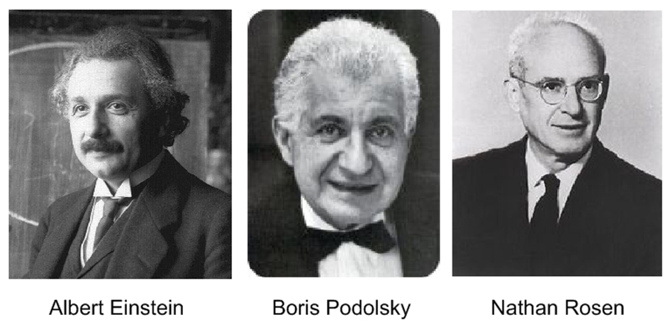
[1] A. Einstein, B. Podolsky, and N. Rosen, “can quantum-mechanical description of physical reality be considered complete?” Phys. Rev. 47, 777 (1935).
[2] JS Bell, “On the Einstein Podolsky Rosen paradox,” Physics 1, 195 (1964).
[3] A. Aspect, P. Grangier, and G. Roger, “Experimental Realization of Einstein-Podolsky-Rosen-Bohm Gedankenexperiment: A New Violation of Bell’s Inequalities,” Phys. Rev. Lett. 49, 91 (1982).
[4] “I am at all events convinced that He does not play dice,” The Born-Einstein Letters, with comments by M.Born, Walker, New York (1971).
[5] “We often discussed his notions on objective reality. I recall that during one walk Einstein suddenly stopped, turned to me and asked whether I really believed that the moon exists only when I look at it.” A.Pais, Rev. Mod. Phys. 51, 863 (1979).
[6] “I cannot seriously believe in the quantum theory because it cannot be reconciled with the idea that physics should represent a reality in time and space, free from spooky actions at a distance.” The Born-Einstein Letters, with comments by M.Born, Walker, New York (1971).

Plaats een reactie