The armchair quantum physicist

---

Spooky action at a distance”, or more formally non-locality, is one of the (or maybe even the) most intriguing and defining aspects of quantum physics. The idea that our world could be non-local is almost a century old. It started around 1935 when Einstein posed his EPR paradox. Today, science is still exploring the consequences and limitations of this non-locality. This post uses a toy model to understand why our world is non-local. We will also discover that Nature poses a limit to non-locality.

For a definition of non-locality, we follow Valerio Scarani [1]:

Non-locality: There exist in nature channels connecting two (or more) distant partners that can distribute correlations that can neither be caused by the exchange of a signal (the channel does not allow signaling, and moreover, a hypothetical signal should travel faster than light) nor be due to pre-determined agreement (because the correlations violate the so-called” Bell’s inequalities”).

Obviously, in our daily lives, we do not experience any non-locality. So, quantum mechanics is more non-local than classical theories. The only known” channel” that distributes non-local correlations are” entangled quantum particles” [1]. Still, the non-locality in quantum mechanics is not unlimited. Tsirelson proved in 1980 in his famous paper that non-locality in quantum mechanics is limited. Quantum effects can be non-local but cannot be “too non-local.”

The Alain Aspect experiment

As a metric for non-locality we use the CHSH correlation [2] (for an introduction of CHSH, see our earlier post). The experiment we have in mind is the Alain Aspect experiment, where one pair of entangled photons is distributed to two observers (who are at different locations). These observers can choose to perform a measurement T or a measurement S on their photons. The outcomes of these measurements are either 1 or -1, and for the individual observer, the results will appear totally random. Suppose the correlation between their results violates the Bell inequalities and cannot be caused by communication. In that case, we must conclude that we are observing non-local effects.

The CHSH inequality is formulated as

2√2 ≤ CHSH ≤ 2√2

where

CHSH = <SS> + <ST> + <TS> — <TT>

Here <ST> denotes the expectation value for a measurement S by the first observer and a measurement T by the second observer.

In the Alain Aspect experiment, the T and S measurements correspond to measuring at different polarization orientations. The maximum violation of Bell’s inequalities occurs when the angle between measurement T and S for each photon is 45 degrees [3]. The relative polarization angle between the two photons is always 22.5 degrees, except in the case that for both photons the T measurement is used. In that case, the relative polarization angle should be 67.5 degrees.

Below, with limited math, we will show in some depth how we can use the formalism of quantum mechanics to calculate the value of the CHSH correlation (which, for specific settings, violates Bell’s inequalities). We will take the angle of the polarization direction as

• First photon. S: polarization at π/4, T: polarization at 0
• Second photon. S: polarization at θ, T: polarization at θ + π/4

We expect to find that the violation of Bell’s inequalities is at its maximum for θ equal to π/8, as this was the setting used by Alain Aspect in his experiments [3].

After deriving this result, looking at the maximum violation of Bell’s inequality for entangled photons is a small step. This leads to Tsirelson’s bound, which poses a limit to the non-locality in quantum mechanics [4]. Tsirelson’s bound has triggered a wide range of research on the foundations of quantum mechanics in the past decades.

Quantum mechanics is, to a large extent, a mathematical formalism. When explaining quantum concepts without math, we must ‘invent’ words to describe these concepts. These words can sometimes obtain a meaning beyond their mathematical origin. This post explains quantum mechanical concepts with limited math (a basic high-school-level understanding of sine and cosine functions should be enough). The calculations below are incomplete, and more would need to be done for a ‘proof’ of any statement. Still, the ambition is to bring the reader a little bit closer to what makes quantum mechanics quantum mechanics.

Quantum mechanics

In quantum mechanics, we describe a system’s state by the wavefunction and represent physically observable quantities by an ‘operator.’ If we apply the operator to the state, we get a probability distribution for the different outcomes we can find when measuring the observable. This sounds abstract, so let’s make it tangible with photon polarization.

We will only look at linear polarization to keep the math as simple as possible (this removes the need to use complex numbers).

Polarization as a vector

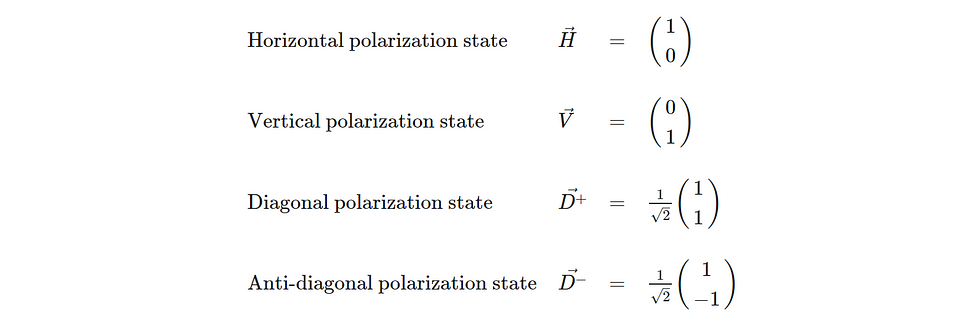
We can describe the polarization of light as a vector. For instance, we can write a vector horizontal polarization and an orthogonal vector vertical polarization. Then, we can also express diagonal and anti-diagonal polarization. We can call the polarization vector the state of a photon.

We can write the state for a photon polarized parallel and orthogonal to a direction specified by an angle θ.

We can express the state for a photon polarized in direction θ in the horizontal and vertical polarization states we defined before.

Note that this post leaves out elliptical or circular polarization to keep the math as simple as possible.

Observables as a matrix

When we measure polarization, we split the two orthogonal polarization directions towards two different detectors. We can, for instance, send a horizontally polarized photon to one detector and a vertically polarized photon to another. A diagonally polarized photon would be equally likely to end up in either detector.

We can also perform a polarization measurement, splitting the diagonal and anti-diagonal polarization into two different detectors. In that case, a horizontally or vertically polarized photon would be equally likely to end up on either detector.

Detecting the photon on either detector would be equivalent to detecting a coin ‘heads up’ or ‘tails up.’ We could compare horizontal polarization to heads up and vertical polarization to tails up. We cannot stretch this analogy to diagonally polarized light. It would require seeing the coins heads up and tails up simultaneously. Even if we considered the coin to be balancing on its edge, the analogy with quantum mechanics would break.

We can describe this measurement with a 2×2 matrix, indicating which polarizations go to either detector. This matrix represents the observable in quantum mechanics. For this post, we use the convention that if we split between horizontal and vertical polarization, we call it the H measurement. In contrast, if we split between diagonal and anti-diagonal polarization, we call it the D measurement. For the H observable, a horizontally polarized photon should give a ‘1’ as a result, and a vertically polarized photon should give a -1. Similarly, we find a 1 or -1 for (anti-)diagonally polarized light with the D observable. This is the case, as we will see in the next section, where we discuss the expectation value of measurement results.

Expectation value of the measurement result

To get to the expectation value of a measurement result for a given state, we have to combine the vector representing the state and the matrix representing the observable. We take the product of the transpose of the state vector (the state vector written as a row instead of a column), the observable, and then again the state vector in column form. In a way, we ‘sandwich’ the observable between the state vectors.

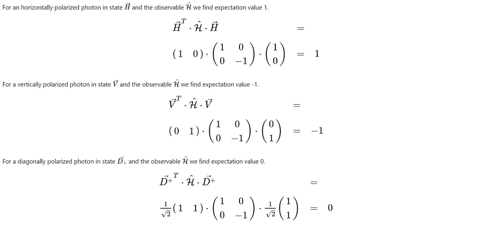
So we see that, as expected, we find the expectation value ‘1’ when measuring a horizontally polarized state with the H observable. The outcome of any individual measurement is either ‘1’ or ‘-1’. If the expectation value is ‘1’, we know that this can only mean that for every individual measurement, we get the outcome ‘1’.

When measuring the vertically polarized state with the H observable, we get an expectation value of ‘-1’. This means that the outcome of every measurement must be ‘-1’.

For (anti-)diagonally polarized light, we find the expectation value ‘0’. This means we are as likely to find the outcome ‘1’ as the outcome ‘-1’ for an individual measurement.

Consecutive measurements on one photon

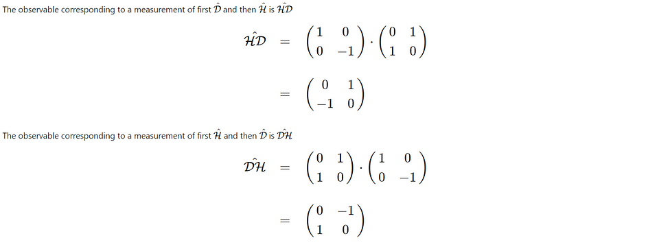
We can multiply the matrices for observables to create a new observable representing consecutive measurements. For example, if we measure D and then H, the new observable would be HD. If we measure the other way round (first H and then D), the new observable is DH (we use it as a convention to write the order from right to left).

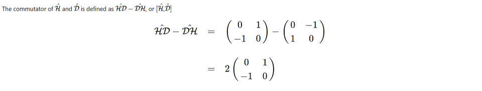
In this case, we see that HD — DH is not zero. In quantum mechanics, we say that the two observables do not commute. This means that it is impossible to assign a definite value to the two observables simultaneously. We can measure H and accept that the value for D is fundamentally unknown. Or we can choose to measure D and leave H unknown. We cannot determine both for one photon. A more exact phrasing of the statement is that the two observables share a Heisenberg uncertainty relationship. What we will see later on is that the fact that the H and D observables do not commute is crucial to getting to a violation of Bell’s inequalities.

Combining sub-systems in one global system

Above we showed how quantum mechanics describes (the measurement of) a single photon. Since we want to explore non-locality, we have to extend our toolbox with additional capability: We have to describe a system with two photons that we measure independently. The ‘tensor product’ in quantum mechanics combines two sub-systems. The symbol for the tensor product is ⊗. We need this symbol to see the difference between multiplying observables for one photon (to represent consecutive measurements) and the observables for different photons (to represent a system consisting of sub-systems). For our toy system, it is sufficient to see this as a way to combine the two photons and their surroundings so that observables only act on photons within their sub-system.

A state with one vertical and another diagonally polarized photon can be written as follows.

If we measure this state with H on the first photon and D on the second photon we get the expectation value for the joined outcome (i.e., the correlation) <H⊗D>.

Entangled states

An entangled state is a state which, by definition, cannot be written as the product of the states for the separate sub-systems. An example of an entangled state would be the state where both photons have the same polarization. We cannot split this state into a state for photon one and a state for photon two. The polarization of the individual photons is not defined. Only the global state of the two photons combined is specified. This will lead to the effect that any measurement of an individual photon leads to a random outcome (whether you measure this photon in horizontal, vertical, diagonal, or anti-diagonal polarization, you will always have a 50% chance of detecting the photon.) This randomness of the individual photon as part of an entangled state is crucial. Without this randomness, we would not be able to observe non-locality.

In the experiment we have in mind the second photon will be rotated over an angle θ.

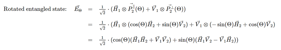
The CHSH observable

Earlier in this post, we phrased the CHSH inequality as 2√2 ≤ CHSH ≤ 2√2, with CHSH = <SS> + <ST> + <TS> — <TT>. To analyze this quantum mechanically, we have to create an operator for CHSH and evaluate the expectation value for this operator for the two-photon entangled state form the previous paragraph.

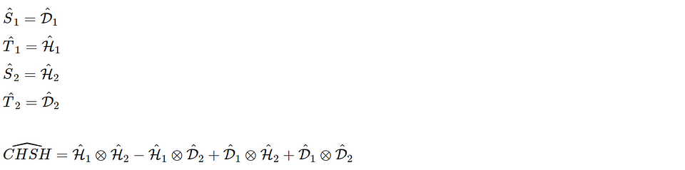
We can define the CHSH observable based on T and S measurements on the respective photons.

We now define the measurements T and S in terms of polarization measurement in horizontal or vertical direction. The rotation θ in the definition of the entangled state, so we define the T and S measurement as:

• First photon. S: polarization at π/4, T: polarization at 0
• Second photon. S: polarization at 0, T: polarization π/4

This leads to

The expectation value for the CHSH correlation is then calculated for the entangled state with the 2nd photon rotated over angle θ.

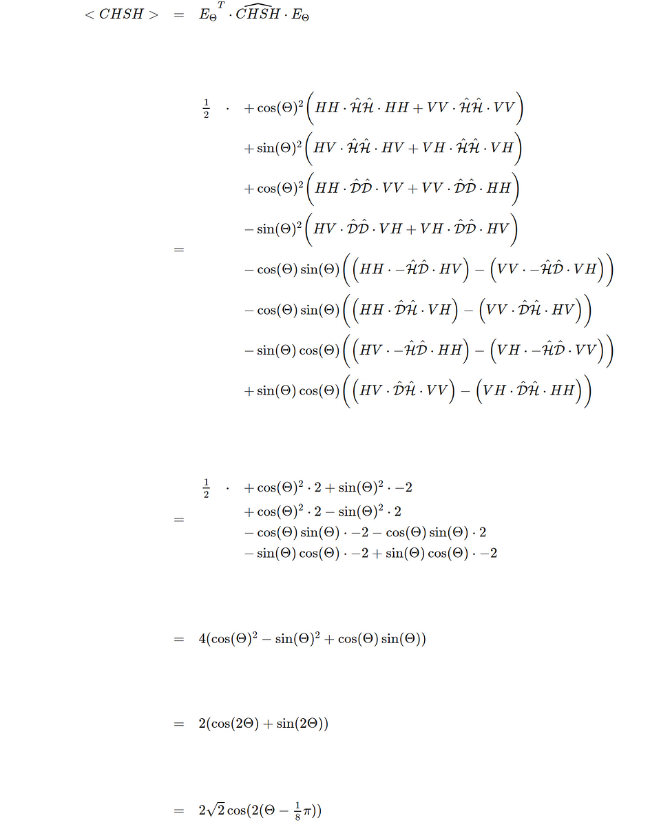
In the final step, we applied the Harmonic Addition Theorem [5]. We see that the maximum expectation value for CHSH correlation is 2√2 (around 2.8). We observe this maximum if we rotate the second photon over an angle of π/8, or 22.5 degrees. This result is very close to the experimental observation of Alain Aspect in his experiments. He observed the CHSH correlation to be 2.7 at the orientation angle of 22.5 degrees between the two photons.

The quantum mechanical calculation presented above might seem tedious, but it is not very complex. We used basic trigonometry and basic manipulation of 2×2 matrices and 2×1 vectors. It is intriguing how this mechanism can lead to something as profound as non-locality. An obvious question is whether this value of 2√2 is the maximum violation of Bell’s inequalities we can find or whether there would be an experiment leading to higher values. After all, once we give up on locality as a requirement, we could imagine the CHSH correlation as high as four from a purely algebraic perspective.

Tsirelson’s bound

In the calculation above, we started with a well-defined state (the entangled state with the second photon rotated) and well-defined observables for both photons (we took H to measure horizontal/vertical polarization and D to measure diagonal and anti-diagonal polarization). In the next step, we will calculate the maximum value of the CHSH correlation for any input state. Calculating the maximum value of the CHSH correlation starts with the notion that the square of an average value of some randomly varying parameter is always smaller than the average value of the square of this parameter.

So, we will calculate the expectation value of the square of the CHSH operator for any input state. From the expectation value of the square, we can then derive the upper bound for the expectation value of the CHSH correlation itself. This bound will be the Tsirelson bound, which can be proven for quantum physics in general (so it has validity far beyond the toy system of two photons, which we study in this post).

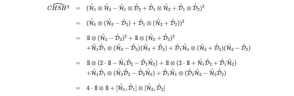
Here, we introduced the ‘identity’ observable which always gives a measurement result ‘1’ for any input state. We also used the idea that the square of an observable will always be the ‘identity.’ Finally, we used the notation for the ‘commutator’ introduced before ([H,D] = HD — DH).

From the description of the square of the CHSH value as observable, we can derive the expectation of this value in an actual experiment. The identity operators will have an expectation value of ‘1’ irrespective of the input state. So, the value of the commutators for the two photons determines the expectation value of CHSH.

We now have derived the expectation value for the square of the CHSH correlation. This gives us an upper bound to the CHSH correlation we can observe independent of what photon state we use in the experiment.

• If the observables used to measure the photons at either side commute (i.e., if they do not share an uncertainty relationship), the values in the square brackets ‘[]’ are zero. Then CHSH² cannot exceed 4, so the CHSH correlation itself has to fall in boundaries set by Bell’s inequalities. Even with an entangled state, the individual photons’ local measurements must fulfill this criterion. Non-commutating observables are a characteristic of quantum mechanics, and in the classical limit, these commutators would be zero. This means that irrespective of any statement on entanglement, we already concluded that a classical theory cannot violate Bell’s inequalities from the properties of these observables.
• Each observable for photon detection has an expectation value that will not exceed 1. The observables correspond to detecting a photon behind a polarizer, and the probability of detecting this photon will not exceed 100%. For this reason, it is reasonable that the maximum value for the commutator [H,D] = HD — DH would be 2. To reach this value, we would need perfect anti-commutations (HD = — DH) and the expectation value for HD to be equal to 1. If we take for the commutators in the above equation this maximum HD. Tsirelson has shown that this upper limit is valid for all of quantum mechanics and that the CHSH correlation within quantum mechanics cannot exceed √8 (=2√2) [4]. So, already in our toy model of two entangled photons, we achieve the highest possible value for the CHSH correlation and the maximum violation of the Bell inequalities.

Superquantum

With the CHSH correlation, we can identify different levels of non-locality. If the CHSH value is not higher than 2, we know we can explain the effect by a “local” theory. We do not violate Bell’s inequalities and can assume that ‘local hidden variables’ carry all the information needed to generate the correlation. If the CHSH value is not above the Tsirelson limit (so not higher than 2√2), we know we can explain the effect by an entangled quantum system (as we observe in the experiment by Alain Aspect). If we ever observe correlations between 2√2 and the algebraic maximum value of 4 for the CHSH correlation, we know quantum mechanics cannot explain it.

The insight that correlation values above the Tsirelson bound are conceivable but beyond quantum mechanics has triggered new research. Why would Nature limit non-locality? Would this level of non-locality violate the theory of relativity? Are there arguments in information theory to explain this limit? In upcoming posts, we will address this research. For now, we conclude that there is space beyond quantum mechanics! Please leave your comments and builds.

---

[1] V. Scarani,” Feats, Features and Failures of the PR‐box,” AIP Conf. Proc. 844. 309 (2006). https://doi.org/10.1063/1.2219371

[2] J. F. Clauser, M. A. Horne, A. Shimony, and B. A. Holt, “Proposed Experiment to Test Local Hidden-Variable Theories” Phys. Rev. Lett. 23, 880 (1969).

[3] A. Aspect, P. Grangier and G. Roger, “Experimental Realization of Einstein-Podolsky-Rosen-Bohm Gedankenexperiment: A New Violation of Bell’s Inequalities,” Phys. Rev. Lett. 49, 91 (1982).

[4] B. Tsirelson, “Quantum generalizations of Bell’s inequality,” Letters in Mathematical Physics 4, 93, (1980).

[5] https://mathworld.wolfram.com/HarmonicAdditionTheorem.html