The armchair quantum physicist

In quantum mechanics, entangled photons show correlations, which can only be explained by what Einstein called ‘Spooky action at a distance.’ Entanglement was ‘discovered’ in the 1930s and first experimentally demonstrated for photons in the 1950s [1]. In the early days, a debate raged in science about whether one could explain these correlations through ‘local hidden variables’ or whether one needed to accept non-locality (i.e., the instantaneous effect of a measurement result at one place on the probability distribution for a measurement at another location). This debate was concluded in the 1980s when Alain Aspect provided experimental evidence for the non-locality of quantum mechanics [2].

Around the time that Alain Aspect published his results proving non-locality, Boris Tsirelson published his work on the limitations of non-locality in quantum mechanics [3]. Tsirelson stated that the non-local correlations in quantum mechanics could not exceed a specific value, known as the Tsirelson bound. Initially, scientists suspected that the Tsirelson bound was linked to the theory of relativity. Relativity theory states that information can not travel faster than the speed of light; potentially, that would also limit non-local correlations.

Sandu Popescu and Daniel Rohrlich demonstrated in 1994 that relativity theory could not explain the Tsirelson bound [4]. They showed that we can conceive non-locality beyond quantum mechanics (i.e., with correlation beyond the Tsirelson bound) that are all perfectly compatible with relativity theory. This triggers the question of why quantum mechanics limits non-locality. What would go wrong if Nature exceeds the Tsirelson bound? What would be the ‘implausible consequences of superstrong non-locality’ [5]?

This post builds on the ideas launched by Sandu Popescu and Daniel Rohrlich. We will modify the entanglement between photons to show ‘superquantum’ behavior. In reality, we cannot create ‘superentangled’ photons, but we will model their behavior in Python. We use the FockStateCircuit package (see the GitHub repository) developed to model quantum optical experiments (like quantum teleportation or the original Alain Aspect experiments) [6].

Entangled photons

The toy model used when studying non-locality consists of two photons entangled in their polarization state. Any polarization measurement on one of the photons gives a totally random result. Still, once one photon is measured, we know the probability of detecting the second photon for a given polarization direction.

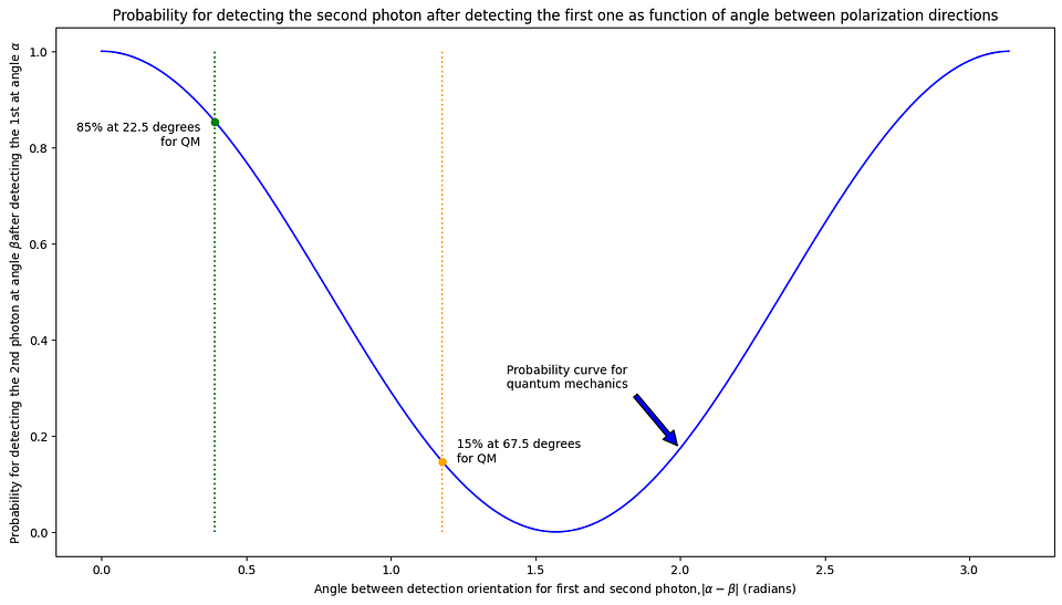
The function P(β|α) is the probability of detecting the second photon at a polarization angle β, given that we detected the first photon at a polarization angle α. P(β|α) = cos(α-β)² for quantum mechanics. Note that the probability only depends on the difference between the angles.

The correlation used is the CHSH correlation [7], which cannot exceed 2√2 for quantum mechanics.

-2√2 ≤ <SS> + <ST> + <TS> – <TT> ≤ 2√2

Here, S and T represent measurements on the photons. The correlation <ST> follows from the P(β|α) if measurement S is at polarization angle α for photon one and T at polarization angle β for photon two.

<ST> = 2P(β|α) — 1

If P(β|α) = 1, we always detect photon two in polarization β after detecting photon one in polarization α, and the correlation <ST> is 1. If P(β|α) = 0, we never see the second photon in polarization β after seeing photon one in polarization α, and the correlation <ST> is -1. If P(β|α) = 50%, the measurement of the second photon in polarization direction β is fully random, and <ST> is 0.

The EPR experiment

We must select specific angles α and β to demonstrate non-locality with two entangled photons. In a previous post, we calculated these angles (also those used for the Alain Aspect experiments).

For the first photon of the entangled pair, we take T to be horizontal polarization (α = 0 degrees) and S diagonal (α = 45 degrees). For the second photon, we take β = 22.5 degrees for S and β = 67.5 degrees for T. With these choices,

• For SS, TS, and ST, we find |α-β| equal to 22.5 degrees; P(β|α) equals (2+√2)/4 ≈ 85%, and <SS>, <TS>, and <ST> are equal to ½√2.
• For TT, |α-β| is equal to 67.5 degrees; P(β|α) equals (2-√2)/4 ≈ 15%, and <TT> is equal to -½√2.

For the CHSH correlation, we find a value precisely at the Tsirelson bound for the specific polarization angles we selected.

CHSH = <SS> + <ST> + <TS> – <TT> = 2√2

In this graph, the probability distribution P(β|α) is plotted as a function of the difference in detection angle α-β between the photons. The green dotted line shows the angle difference for correlations SS, TS, and ST, while the orange dotted line shows the angle difference for correlation TT.

Superentangled photons

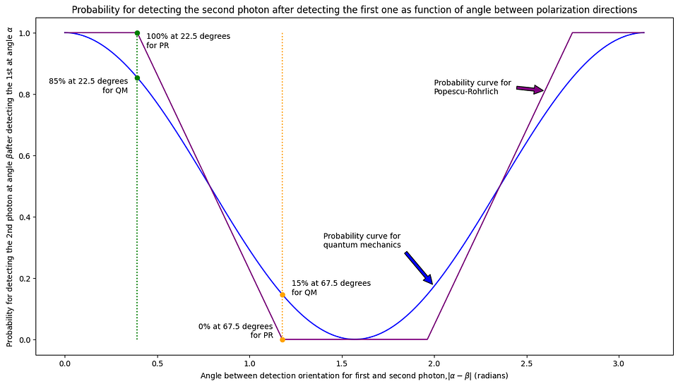
The insight from Popescu and Rohrlich was that we can assume another probability distribution leading to higher correlations. Specifically, they proposed a probability distribution where P(β|α) = 1 if α-β ≤ 22.5 degrees and 0 if P(β|α) = 0 if α-β ≥ 67.5 degrees.

The graph below shows the probability distribution from quantum mechanics next to the distribution taken by Popescu and Rohrlich.

For the CHSH, the Popescu-Rohrlich correlation leads to remarkable results.

• For SS, TS, and ST, we find |α-β| equal to 22.5 degrees; P(β|α) = 100%, and <SS>, <TS>, and <ST> are equal to 1
• For TT, |α-β| is equal to 67.5 degrees; P(β|α) = 0%, and <ST> is equal to -1

The CHSH correlation for this probability distribution is equal to the maximum conceivable value of four, which is well above the Tsirelson bound.

CHSH = <SS> + <ST> + <TS> — <TT> = 4

The Popescu-Rohrlich photons show ‘superquantum’ behavior. Note that individually, these photons still behave as ‘normal’ photons. The only change we made is in their entanglement properties.

Superquantumness as a parameter

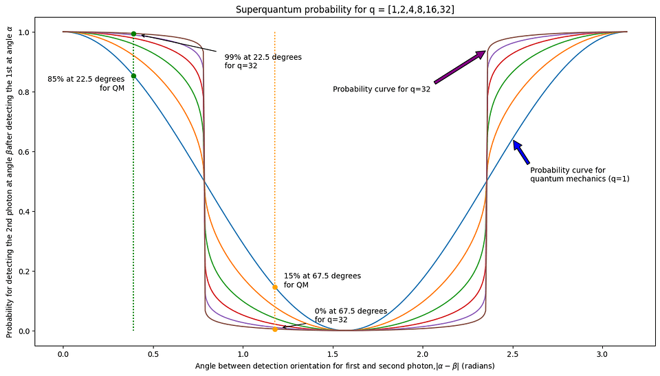
Popescu and Rohrlich propose one probability distribution leading to the maximum non-locality conceivable. We can also consider a gradual transition from quantum mechanics into superquantum correlations. We introduce a ‘superquantumness’ parameter q, which can take a value of 1 or higher. For q=1, the entanglement is quantum mechanical, and for the limit q to infinity, we obtain the Popescu-Rohrlich correlation. The probability distribution we take to achieve this is based on higher-order roots.

When we plot the probability distribution for different values of q, we see the gradual transition from the quantum domain to the Popescu-Rohrlich correlation with increasing q.

Optical experiments with ‘superentangled’ photons

We have generalized the Popescu-Rohrlich concept for superentangled photons. By varying the ‘superquantumness’ parameter q, we can tune from regular quantum behavior at the Tsirelson bound to the highest conceivable correlations expected for Popescu-Rohrlich photons. We run these experiments using the FockStateCircuit package in Python [6].

We will first run two photon pairs through a simple optical set-up with half-wave plates. One pair will have a q-value of 1, and the other will have a q-value of 5. After the wave plates, we detect the photons to determine the correlation. We score ‘1’ if we detect both photons with the same polarization and ‘-1’ if we see them with orthogonal polarization. This picture summarizes the setup.

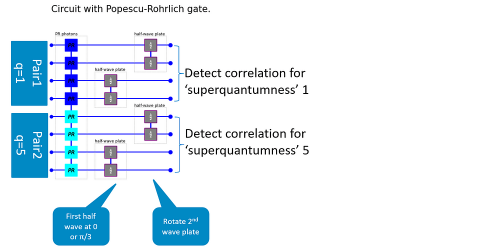
What do we expect to find?

1. If the half-wave plates are aligned, we expect perfect correlation, and if the wave plates are at an angle of 45 degrees, perfect anti-correlation. At 22.5 degrees between the wave plates, we expect no correlation. These conditions should hold for all q-values.
2. We expect that the shape of the correlation curve changes for different q-values, reflecting the ‘superquantum’ entanglement.
3. If we change the detection for the first photon (by rotating the half-wave plate for that photon), we expect to see a shift for the second photon as well.

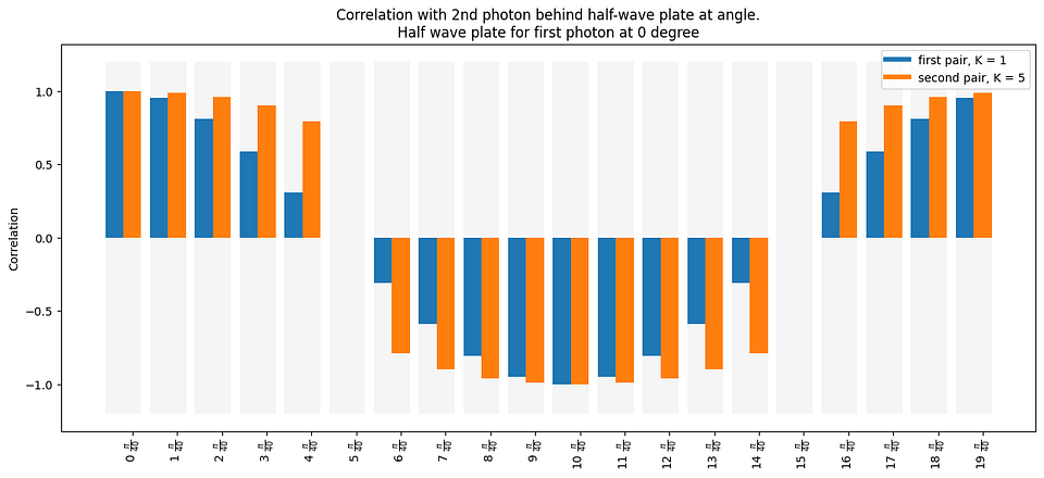
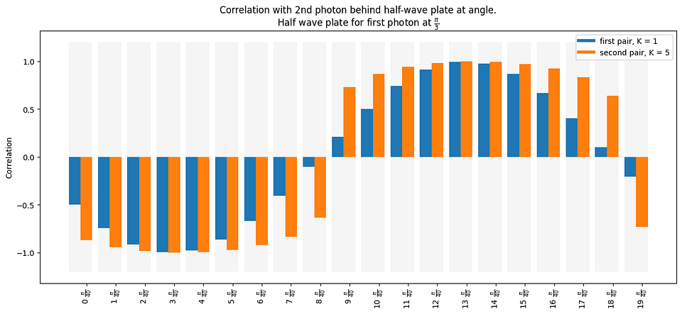
These graphs above show in blue the correlation for the photon pair with regular entanglement and in orange the correlation for the ‘superentangled’ pair. If we change the half-wave plate for the first photon, we see the expected behavior, including the shift in probability distribution for the second photon. In the model, we used regular optical components so the superentangled photons individually behave exactly as a photon; the only difference is in their entanglement.

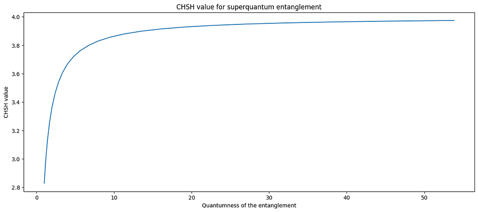
As the next step, we will use superentanglement in the EPR/Alain Aspect experiment. We create a photon pair and send the photons to two observers. They can do a T or an S measurement. For the entangled photons, S and T correspond to polarization detection at 45 degrees and 0 degrees for the first photon and 22.5 degrees and 67.5 degrees for the second photon. The CHSH value will be the correlation <SS> + <ST> + <TS> – <TT>. For regular photons, this CHSH value cannot exceed 2√2, for ‘superentangled photons’, we expect to see CHSH correlation up to a value of four.

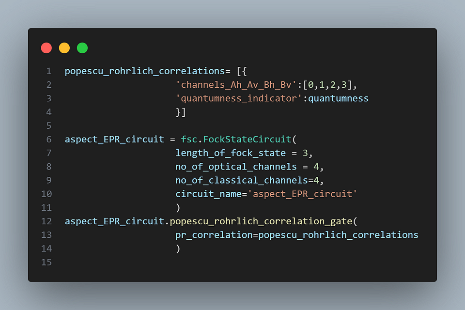
We use the same EPR optical circuit as in the FockStateCircuit tutorial [8]. The change we made is that we added ‘no-signaling boxes’ as input states, replacing the regular entangled state. On the output side, we need to evaluate the result with a dedicated function to capture the result. The code snippet below shows how these functions are called (for the complete code, see GitHub for the Jupyter Notebook belonging to this post).

We see that, as expected, the CHSH correlation approaches the maximum value of four for increasing q-values. So, our photons show correlations well above the highest value possible in quantum mechanics when measured on the same optical setup used for regular photons.

Why is Nature not superquantum?

In this post, we discussed Sandu Popescu and Daniel Rohrlich’s work. They conceived photons showing ‘superentanglement’. These photons will break the Tsirelson bound for CHSH correlation, so they are not possible in quantum mechanics as we know it.

Popescu and Rohrlich showed that relativity theory does not lead to the Tsirelson bound. The ‘superentangled’ photons do not require faster-than-light communication. The same non-locality that is needed for regular entanglement could also enable superentanglement. This post showed that ‘super entangled’ photons can still behave as photons. They have the same behavior for optical components like beamsplitters or wave plates. So, in principle, superentanglement is possible. So, why does quantum mechanics limit non-locality? What would go wrong if Nature exceeded the Tsirelson bound?

The following posts will address this question from another perspective and explore what happens if we use superentangled particles as a resource for communication and information processing. Finding a structural difference between regular and super-entanglement for communication and information processing can shed new light on the upper limit for quantum correlations. Potentially, we can use information-theoretical arguments as a physical principle.

---

[1] C. S. Wu and I. Shaknov, “The angular correlation of scattered annihilation radiation,” Phys. Rev. 77, 136 (1950).

[2] A. Aspect, P. Grangier and G. Roger, “Experimental Realization of Einstein-Podolsky-Rosen-Bohm Gedankenexperiment: A New Violation of Bell’s Inequalities,” Phys. Rev. Lett. 49, 91 (1982).

[3] B. Tsirelson, “Quantum generalizations of Bell’s inequality,” Letters in Mathematical Physics 4, 93, (1980).

[4] S. Popescu and D. Rohrlich, “Quantum Nonlocality as an Axiom,” Foundations of Physics 24, 397 (1994).

[5] W. van Dam, “Implausible consequences of superstrong nonlocality,” Nat Comput 12, 9–12 (2013).

[6] For the package see https://github.com/robhendrik/FockStateCircuit (or install on PyPi https://pypi.org/project/FockStateCircuit/. For the code used in this blogpost see https://github.com/robhendrik/Popescu-Rohrlich-photons

[7] J. F. Clauser, M. A. Horne, A. Shimony, and B. A. Holt, “Proposed Experiment to Test Local Hidden-Variable Theories” Phys. Rev. Lett. 23, 880 (1969).

[8] See the notebook fock_state_circuit_tutorial.ipynb on Github (https://github.com/robhendrik/FockStateCircuit/tree/main/docs)