The armchair quantum physicist

Quantum non-locality is the effect that there can be a strong correlation between events at distant locations. Scientists have performed experiments where they observe these correlations and can exclude any communication or otherwise shared information that causes them. The correlations exist because Nature is fundamentally non-local.

In the 1980s, Boris Tsirelson demonstrated that non-locality in quantum mechanics has an upper bound [1]. Tsirelson based his argument on quantum mechanics’ mathematical formalism. Scientists wondered whether there was a high-level principle explaining this upper limit, which is called the ‘Tsirelson bound.’

In 1994, Sandu Popescu and Daniel Rohrlich presented their work on ‘superphotons’ [2] (see also our earlier post). These photons behave like ordinary photons except for their entanglement properties. For two entangled photons, the angle between the polarization directions determines the likelihood of their detection. If we measure one photon in polarization direction α and the second in polarization direction β, the probability of detecting the photons is cos(α-β)². Popescu and Rohrlich proposed (as a thought experiment) to change this relation such that the probability would be 1 if the difference between α and β is smaller than 22.5ᵒ and 0 if the difference is larger than 67,5ᵒ. They demonstrated that these photons exhibit non-locality beyond the Tsirelson bound but do not violate any other physical principle. Specifically, they concluded that these photons are fully compatible with Einstein’s relativity theory because no actual information is transmitted faster than the speed of light.

So, after the work of Tsirelson and the analysis by Popescu and Rohrlich, we are left with the situation that we can calculate that there is an upper limit to quantum non-locality, but we cannot truly understand it. If the difference between an ordinary photon and a ‘super photon’ is so tiny, and if these super photons are fully compatible with any known physical principle, why would these ‘super photons’ not exist? What would be the higher-level principle from which we can derive the Tsirelson bound?

Guessing game

In the 1990s, Marcin Pawłowski and co-workers introduced a guessing game [3]. In this game, we have two players (Alice and Bob). Alice has some information (it can be a CD with music or a few movies on a hard drive). It is Bob’s task to guess this information. The success rate in the game is the percentage of cases where Bob can guess successfully. Alice is only allowed to communicate a certain amount of information to Bob. Bob’s chance of guessing correctly will grow if Alice is allowed to share more information with Bob.

To model the game, we represent Alice’s information as a string of bits. Let’s assume she has a string of 8 (random) bits, like ‘10010110’ or ‘00110011’. Bob will get the task of guessing the value of one specific bit in Alice’s bitstring. For instance, we ask Bob to guess the first or third bit. Bob’s success rate would be 50% if Alice would not share any information. If Alice would share 8 bits, Bob’s success rate would be 100% (because he would know the value of Alice’s bits completely).

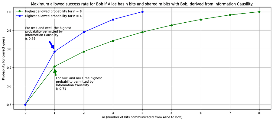
In Figure 1 below, we show the maximum allowed success rate for Bob in the situation that Alice has a bitstring of length n=4 or n=8 for different values of m (m is the amount of classical bits shared representing the amount of communication). Bob’s success increases from 50% if he does not receive any information to 100% if he receives the total amount of information representing Alice’s bitstring. These success rates represent the highest probability ‘allowed’ in information theory, given the amount of information shared between Alice and Bob. If Bob and Alice have a flawed algorithm or make mistakes, their success rate will be lower. The figure is the maximum they can obtain.

In the next step, Alice and Bob are allowed to share entangled (super)photons. We ensure these do not contain any information on Alice’s bit string (for instance, we generate and distribute the photons before Alice’s bit string is known). So, the entangled photons are not a communication channel by themselves. The argument from information theory where Bob’s success rate is limited by the amount of information shared still holds. So, we should not see any success rate above the green (for n = 8) or blue (for n = 4) curves in Figure 1, even if Alice and Bob share entangled photons. If we had higher probabilities, something unnatural would have happened, as Bob would have had more information available than had been shared with him.

We use Python to implement the algorithm proposed by Pawłowski, see GitHub for the Jupyter Notebook. As basis we use the package FockStateCircuit. This package is designed to model quantum optical systems and is ideally suited for this experiment. This package offers the feature to work with ‘superphotons’. We used this in an earlier post where we introduced the Popescu-Rohrlich photons. We can set the entanglement behavior of these photons by a ‘quantumness parameter.’ If this parameter, q, is 1, the photons are regularly entangled (i.e., in practice, we could experiment with real photons). If the quantumness increases, the entanglement properties change. In the limit of the q-value going to infinity, the photons will behave as proposed by Popescu and Rohrlich in their seminal paper. This quantumness parameter can scale from ordinary entanglement to the strongest conceivable superentanglement.

In Pawłowski’s algorithm, Alice performs a series of measurements on the photons at her side. If Alice has a bitstring of length 8, we need seven pairs of entangled photons (where for each pair, one photon is with Alice and one with Bob).

Algorithm at Alice’s side

Based on the values in her bitstring, Alice has to perform a series of measurements on the photons at her side. The algorithm is iterative; she first measures four photons and does some calculations. Then Alice repeats the process with two photons and finally once more with one photon. For each iteration, she generates a new bitstring that is half the size of the original. After the last iteration, Alice has one bit left. This bit she communicates to Bob. So Alice measures seven photons to generate one bit of classical information. Note that for Alice, the value of this bit appears random. Even if she starts with the same bitstring, she has a 50% chance of generating a ‘1’ as the final bit and a 50% chance of generating a ‘0’.

Algorithm at Bob’s side

Bob, at his side, also measures the photons. His measurement strategy depends on the ‘index’ of the bit he has to guess. Bob stores the measurement results and combines them with the bit received from Alice. From this combination, he generates his ‘guess.’

The Python code belonging to the current post (in a Jupyter Notebook on GitHub) describes the algorithm. No complex mathematics is involved, so anyone interested can easily explore and play with this. For this post, we will not go deeper into the algorithm but refer the reader to GitHub.

The circuit

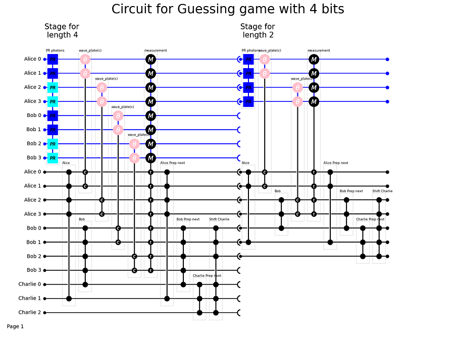
Figure 2 shows our circuit when Alice has a bitstring of length n = 4. The circuit has three ‘stations’: One for Alice, one for Bob, and one for Charlie as an independent referee. Charlie generates the assignment for Alice and Bob and judges whether Bob has guessed correctly.

Now, we execute the algorithm with regular photons. We set the quantumness parameter to one (for q = 1, the photons have ordinary entanglement).

# see GitHub for full code
# https://github.com/robhendrik/Guessing-game-with-superphotons-A-Python-simulation
quantumness=1
bit_string_length = 8

# first generate the circuit
circuit_list = []
bit_string_length_counter = bit_string_length
while bit_string_length_counter > 1:
    circuit =   generate_circuit_for_stage_in_guessing_game(length_of_bitstring=bit_string_length_counter ,quantumness=quantumness)
    circuit_list.append(circuit)
    bit_string_length_counter = bit_string_length_counter //2
compound_circuit = fsc.CompoundFockStateCircuit(list_of_circuits=circuit_list)

# prepare the input state
initial_collection = fsc.CollectionOfStates(fock_state_circuit=circuit_list[0], input_collection_as_a_dict=dict([]))
charlies_number = np.random.randint(0,2**bit_string_length)
bobs_index = np.random.randint(bit_string_length)     
alices_bit_list = number_to_bit_list(charlies_number,bit_string_length)
state = fsc.State(initial_collection)
state.initial_state = str(iteration) + "Expected: " + str(alices_bit_list[bobs_index])
state.classical_channel_values[-3] = bobs_index
state.classical_channel_values[-2] = charlies_number
state.cumulative_probability = 1
initial_collection.add_state(state)

# run the circuit
resulting_collection = compound_circuit.evaluate_circuit(initial_collection)

# to determine success rate we check per state if the last character of the initial_state is '0' or '1' (the initial state
# is the 'Expected: 0' or 'Expected: 1'.). This character we compare to the value in last classical channel (Charlies 3rd channel).
# This channel should contain Bob's guess. If the guess is the same as indicated in the initial_state we add the probability for this
# state to the variable correct, otherwise to the variable fault
fault = 0
correct = 0
for state in resulting_collection:
    guess = state.classical_channel_values[-1]
    if str(guess) == state.initial_state[-1]:
        correct += state.cumulative_probability
    else:
        fault += state.cumulative_probability

# We can simulate the expected outcome. For each state the success rate should be 85%. We expect the correct answer if all stages deliver
# a correct result or if only one of the stages delivers a correct result (two stages with an incorrect result cancel eachother, so together
# they still come to a correct outcome!)
Psuccess = 0.5+0.5*np.cos(np.pi/4)
Pfail = 1-Psuccess
Ptotal = Psuccess**3 + Psuccess*Pfail*Pfail*3
print("Success rate expected for single stage: ", np.round(Psuccess,2), "Expected in total: ", np.round(Ptotal,2))

# Compare what we expect to what we find
print('For a quantumness value of 1 we expect a success rate of', np.round(Ptotal,2),' for the three stages combined')
print('From the simulation we find a value of: ', np.round(correct/(correct+fault),2))

Success rate single stage:  0.85 Expected in total:  0.68
For a quantumness value of 1 we expect a success rate of 0.68  for the three stages combined
From the simulation we find a value of:  0.68

If we run the experiment for q = 1, we see that Bob’s success rate is 68%. This value is below the limit from Figure 1. Despite using entangled photons and this complex procedure, we cannot conclude that Bob’s success rate is surprising. His success is fully compatible with the fact that Alice has sent him one bit of information; from an information theoretical perspective, they could even do a little bit better.

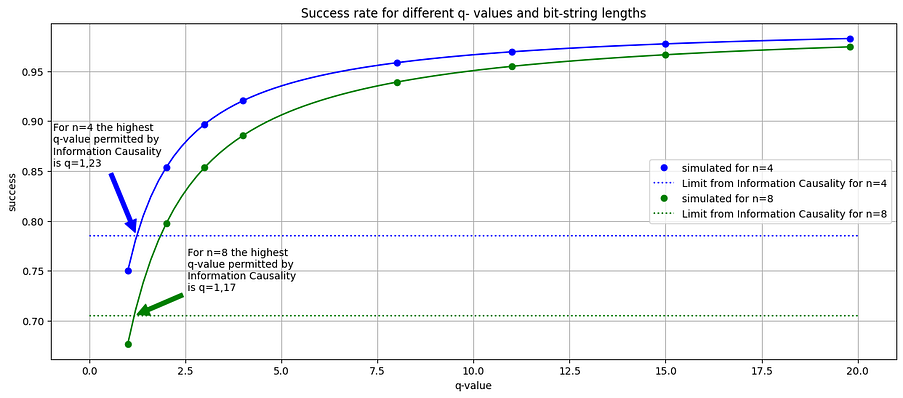
Now, let’s run the experiment with ‘superphotons’. We use quantumness parameters up to 20. Remember that for q=1, the photons behave as ordinary entangled photons, and for very high values, they behave as proposed by Popescu and Rohrlich. We see in Figure 3 that for values just above 1, Bob’s success rate already exceeds what information theory allows. For the higher q-values, Bob’s success rate even approaches 100%. This success depends on communicating just one bit of information, with the help of ‘superentangled’ photons, which do not carry any information on Alice’s but string.

Information Causality

So, suppose we change the entanglement between the photons slightly by increasing the quantumness parameter. In that case, we already see that we can utilize the photons for communication beyond what information theory permits. We would violate a higher-level principle, as information cannot appear out of nowhere. Pawłowski named the principle that Bob cannot utilize more information than he received from Alice as ‘Information Causality.’ With Information Causility, we can explain why Nature limits non-locality in quantum mechanics to the Tsirelson bound since we can easily violate Information Causality with photons that break the Tsirelson bound.

When Alice has 4 or 8 bits, we can use photons with a quantumness value of just above one without violating Information Causality. So, we cannot derive exactly the Tsirelson bound (corresponding to a q-value of precisely one) for these situations. If we increase the bit string at Alice’s side, we will see that the boundary will move closer to q = 1. So, we can define the Tsirelson bound as the level of quantum non-locality, which ensures that for an arbitrary large bit string at the side of Alice, the success rate for Bob will not exceed the maximum value allower from information theory.

Conclusion

This conclusion is striking. When Tsirelson derived the value of ‘his’ bound in the 1980s, he utilized the highly mathematical formalism of quantum mechanics. We can derive this limit from the high-level principle of Information Causality. This triggers the question of whether other fundamental aspects of (quantum) physics also stem from information theory.

In the next post, we will discuss a recent development in a field where Marcin Pawłowski showed that we can also derive the Tsirelson bound by utilizing just one set of entangled (super)photons [5]. In the algorithm we discussed in the current post, we need infinite photon pairs to calculate the Tsirelson bound with high precision. In the next post, we will see that we can achieve the same result with just one photon pair. Until then, please leave your build and comments on this post.

[1] B. Tsirelson, “Quantum generalizations of Bell’s inequality,” Letters in Mathematical Physics 4, 93, (1980).

[2] S. Popescu, D. Rohrlich, “Quantum non-locality as an axiom,” Found Phys 24, 379 (1994). https://doi.org/10.1007/BF02058098

[3] M. Pawłowski, T. Paterek, D. Kaszlikowski, V. Scarani , A. Winter and M. Zukowski, “Information causality as a physical principle,” Nature 461, 1101 (2009). https://doi.org/10.1038/nature08400

[4] The code used for this post can found on GitHub in a Jupyter Notebook ( https://github.com/robhendrik/Guessing-game-with-superphotons-A-Python-simulation) or HTML format (https://robhendrik.github.io/Guessing-game-with-superphotons-A-Python-simulation)

[5] N. Miklin and M. Pawłowski, “Information Causality without Concatenation,” Phys. Rev. Lett. 126, 220403 (2021). https://doi.org/10.48550/arXiv.2101.12710