Beamsplitters and the quantum HOM effect

See the Jupyter Notebook for the Quantum HOM Effect on Github pages.

This is the first post from a series of three on the HOM effect. For the second post see ‘The HOM effect explained’, and for the third post see ‘Simulating the HOM effect on a quantum computer’

Main reference: C. K. Hong, Z. Y. Ou, and L. Mandel, “Measurement of subpicosecond time intervals between two photons by interference”, Phys. Rev. Lett. 59, 2044 – Published 2 November 1987

Introduction

In this notebook we use a very simple optical component: A beamsplitter. We will start by looking at a beamsplitter which leaves half of the light through and which reflects the other half, and later we will vary the reflectance and transmittance.

For single photons we find the expected, and rather boring outcome that the photon either passes through the beamsplitter, or is reflected by the beamsplitter with a probability depending on the reflectance or transmittance of the beamsplitter. For a 50%/50% beamsplitter you would find an input photon with equal likelihood in any of the output ports of the beamsplitter.

However, when using two photons it gets a lot more interesting. We see that when the photons are fundamentally ‘indistinguishable’ an effect occurs leading to the two photons always being together in any of the outputs. This ‘bunching’ is known at the HOM effect, named after Hong, Ou and Mandel (see their paper “Measurement of subpicosecond time intervals between two photons by interference” which is the main reference for this notebook). We will also see that through the HOM effect we can create entanglement and achieve a non-classical correlation between measurement outcomes behind the different output ports of the beamsplitter.

In this notebook we first describe a beamsplitter with the input and output states in such a way that we can easily model it in Python Qutip (see the jupyiter notebook on GitHub pages ). We then define some Python functions as a kind of ‘infrastructure’ to simulate the effect of the beamsplitter. Then we use this model first for single photons, and then for photon pairs. To dive deeper we use a varying polarization to continuously vary the level of ‘indistinguishability’, and also play with the reflectance and transmittance of the beamsplitter.

Outline:

The beamsplitter
Mixing matrices
Setting up the optical system
Measuring statistics with single photons
Measuring statistics with photon pairs
Varying the degree of ‘indistinguishability’
Conclusion

The beamsplitter

We use a simple Qutip model to mimic the actual experiments. In this model we use a 4 channel Fock state for the input and the output. At the input the 4 channels represent the horizontal and vertical polarization at input port 1 and input port 2. So for example the input state |1000> would represent one horizontally polarized photon at input port 1, while |0001> would represent one vertically polarized photon at input port 2. |1010> would represent a horizontally polarized photon at port 1 and port 2 simultaneously, while |0011> would represent a horizontally and a vertically polarized photon both at port 2. For the output the logic is similar: |1000> represents a photon with horizontal polarization at output port 1, while |0020> represents a state with two horizontally polarized photons at output port 2. In this notebook we limit ourselves to 4 channels, and maximum 2 photons in the system.

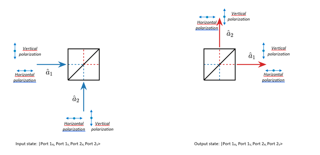
We limit ourselves to the case where the beamsplitter is not polarization dependent, i.e., the situation where the beamsplitter works the same for any polarization at the input ports. We will however vary the polarization of the light between the two different input ports and between the light at the input port and the detectors behind the output port. So, the beamsplitter itself is not polarization dependent, but we will vary the polarization of the input light and the polarization direction of the output detection.

Mixing matrices

Above we discussed how our optical system can be described by a Fock state indicating the number of photons per channel. Modifying this state happens through optical components like beamsplitters, which we mathematically describe by matrices.

Two channels

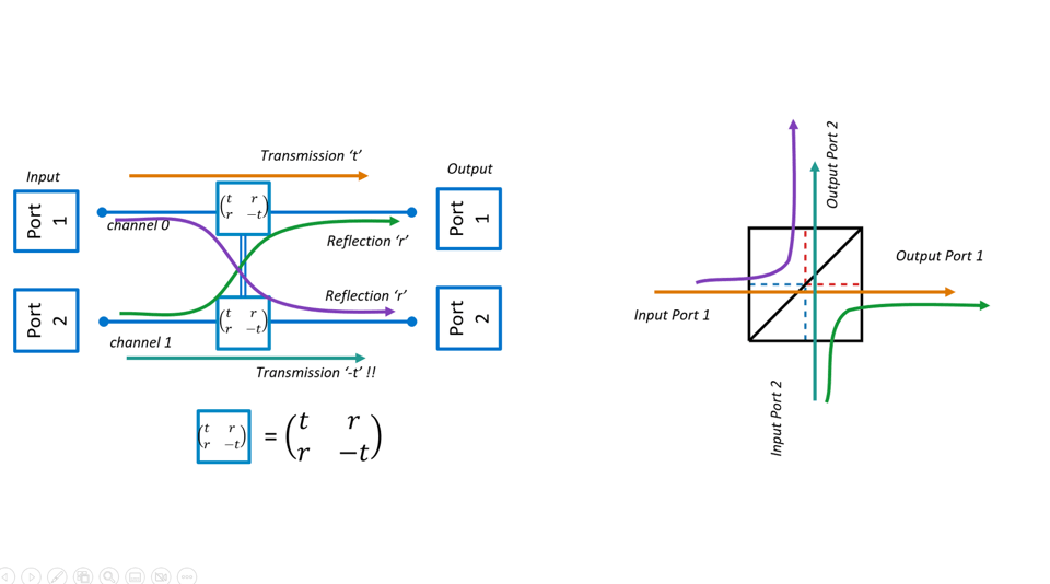
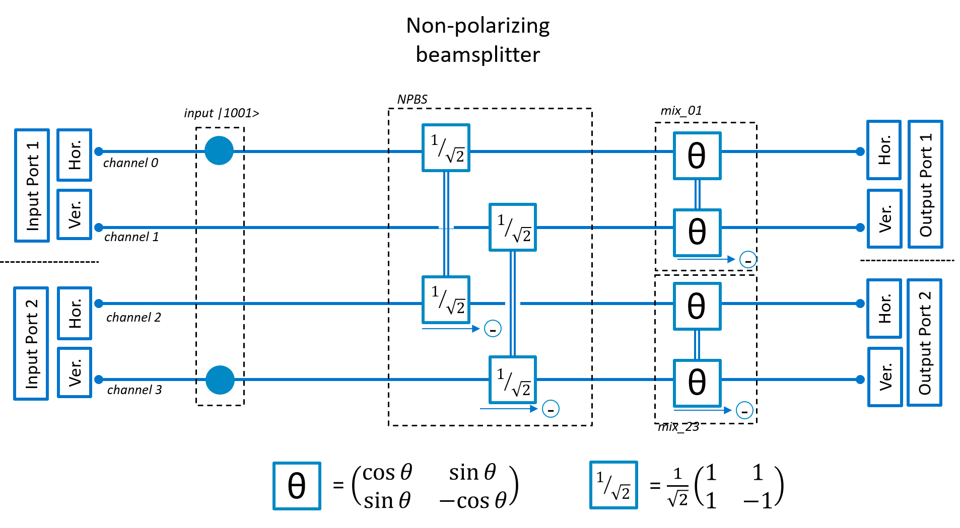
To model the beamsplitter we define the matrix below for mixing two channels. Here the transmission coefficient is t and the reflection coefficient is r. These coefficients act on the ampitudes. So if for instance t=r=1/√2 the probability to be reflected is r²=1/2 and the probability to be transmitted is t²=1/2. So this would be a 50%/50% beamsplitter equally splitting the light between the output ports. Below we see a picture representing this beamsplitter as mixing two channels, where it is important to note the ‘minus sign’ that has to be included for transmission from input port 2 to output port 2.

$\begin{pmatrix} r&t\\t&-r\end{pmatrix}$

So for input state |10> the output state is |rt>, and for |01> the output state is −|tr>

Below an illustration of the beamsplitter as ‘mixing two channels’. Note the minus sign for passing from port 2 input to port 2 input. This will be important!

There are some special cases which we will use further down in this notebook

We can make a ‘swap’ matrix to simply swap the two channels. |10>→|01> and |01>→|10>. In this case we set r equal to zero and t equal to 1.

$\begin{pmatrix}0&1\\1&0\end{pmatrix}$

The 50%/50% beamsplitter we use mostly in this notebook is modelled by using $\frac{1}{\sqrt{2}} = \frac{1}{2} \sqrt{2}$ for both the reflection (r) and transmission (t) coefficient. The matrix then looks like

$\begin{pmatrix}\frac{1}{2}\sqrt{2}&\frac{1}{2}\sqrt{2}\\\frac{1}{2}\sqrt{2}&-\frac{1}{2} \sqrt{2} \end{pmatrix}$

or more clearly

$\frac{1}{2}\sqrt{2}\begin{pmatrix}1&1\\1&-1\end{pmatrix}$

We can also make a beamsplitter with a different ratio between transmission and reflection, as long as |r|² + |t|² = 1 (we still assume the beamsplitter to be lossless, all light that enters comes out somewhere). To use this generic beamsplitter we take the matrix below where r equals $\cos(\theta)$ and t equals $\sin(\theta)$

$\begin{pmatrix}\cos(\theta)&\sin(\theta)\\\sin(\theta)&-\cos(\theta)\end{pmatrix}$

For more information on how to describe a beamsplitter with a matrix check out https://en.wikipedia.org/wiki/Beam_splitter or https://www.pas.rochester.edu/~howell/mysite2/Tutorials/Beamsplitter2.pdf.

Four channels

To generalize the two channel matrices for a 4 channel system we can simply extend the matrix. For instance, for only mixing channels 0 and 1 in a 4 channel system the matrix would be like:

$\begin{pmatrix}r & t & 0 & 0 \\t & -r & 0 & 0\\0 & 0 & 1 & 0 \\0 & 0 & 0 & 1\end{pmatrix}$

Mixing channels 1 and 3 would look like:

$\begin{pmatrix}1 & 0 & 0 & 0 \\0 & r & 0 & t\\0 & 0 & 1 & 0 \\0 & t & 0 & -r\end{pmatrix}$

Setting up the optical system

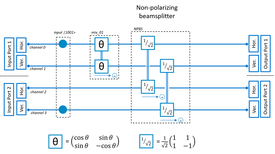
We first look at an optical system with a non-polarizing beamsplitter. The basic setup has horizontal/vertical polarization at the input and horizontal/vertical polarization orientation for the detectors. Optionally we can add an element at the input/output ports to change polarization orientation to diagonal.

Measuring statistics with single photons

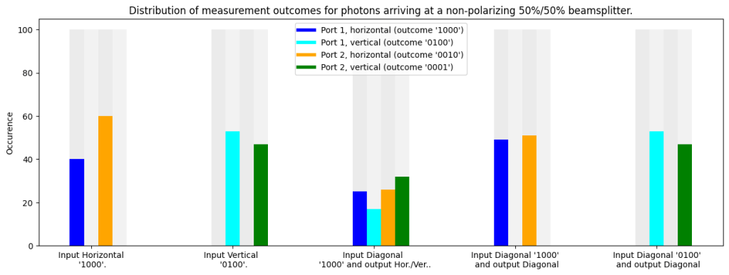
If we start with a horizontally polarized photon at the first input port (input state |1000>) we find at the output 50% change of a horizontally polarized photon behind the first port (outcome ‘1000’), and 50% change on a horizontally polarized photon at the second port (outcome ‘0010’). If we start with a vertically polarized photon (input state |0100>) we find vertical polarization at the output, 50%/50% split between the two ports (outcomes ‘0100’ and ‘0001’).

Starting with a diagonally polarized photon and leaving the detection in the horizontal/vertical polarization leads to finding a photon 50%/50% between the output ports, and also 50%/50% between horizontal and vertical polarization. So in this case all outcomes (‘1000’, ‘0100’, ‘0010’ and ‘0001’) are equally likely.

If we change the detection also to the diagonal direction we again see that polarization is maintained in the beamsplitter.

Measuring statistics with photon pairs

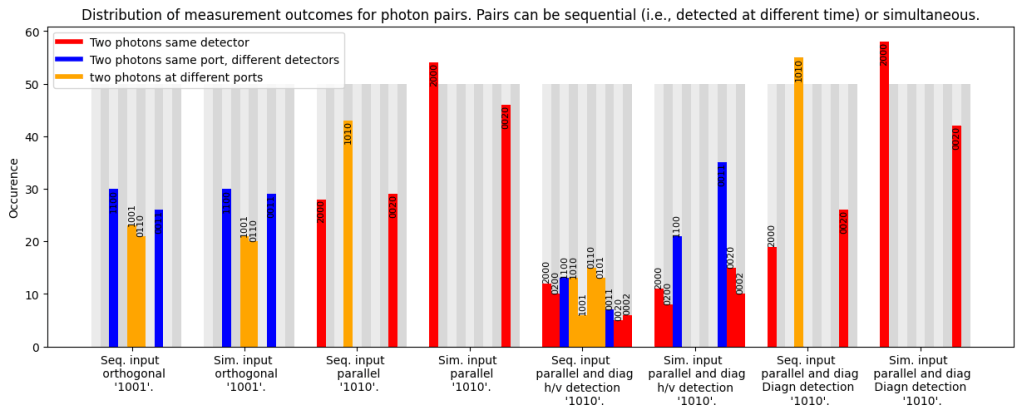
Below we see the statistics in the measurement when using photon pairs, which either arrive sequentially or simultaneously. For the sequential photons we see the same statistics as for the single photons: We always see that polarization is maintained (i.e., 2 horizontally polarized photons at the input always gives two horizonally polarized photons at the output, one horizontally and one vertically polarized photon at the input gives the same at the output). Also, we see that we always have the same occurence of ‘bunching’ (i.e., two photons in one port) as the occurence of ‘anti-bunching’ (i.e., one photon in each output port).

If the photons arrive simultaneously and have a different polarization nothing changes, we still see the statistics observed for sequential photons with the same occurence of ‘bunching’ and ‘anti-bunching’.

If however we have two photons with the same polarization entering the two ports simultaneously we see a special effect. The anti-bunching disappears and the photons only show up together behind one of the output ports. This is the famous HOM-effect, named after Hong, Ou and Mandel.

If we rotate the polarization at the input by 45 degrees to diagonal orientation and also use diagonal polarization at the detectors we also see only ‘bunching’. So clearly the HOM effect does not depend on polarization, as long as the polarization of the photons is the same (and as long as they arrive simultaneously).

Varying the degree of ‘indistinguishability’

Changing the polarization of the input ports to vary ‘indistinguishability’

In literature it is mentioned that the HOM effect is driven by photon ‘indistinguishability’. In the detection statistics we observe in the computer experiments we indeed see that for photons arriving simultaneously (i.e., we cannot identify by their arrival time) we see the HOM effect, while if the photons arrive sequentially (i.e., they come one at a time and could be identified by their arrival time) the effect disappears. The effect also disappears if both photons have different polarization (so if we could identify them by their polarization).

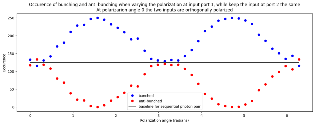
Let’s now look what happens if we rotate the polarization at of the input ports from orthogonal to parallel. In that case we gradually vary the photons from being fully disinguishable to fully indistinguishable. The setup used is given in below diagram.

When we look at the occurence of the measurement outcomes we see that for $\Theta = 0$ there is as much ‘bunching’ and ‘anti-bunching’. This is as expected. When we rotate the polarization at input port 1 we see the occurence of bunching increasing to be fully ‘bunched’ at $\Theta = 90^{o} (\frac{\pi}{2}$ ).

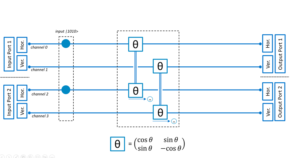
Changing the reflection and transmission of the beamsplitter to vary ‘indistinguishability’

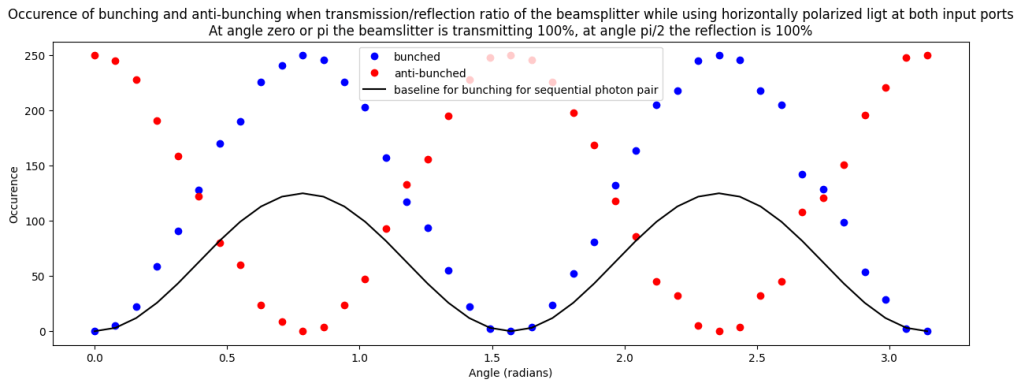
What we can also do is start with parallel polarized photons for the two ports, but vary the reflectivity and transmissivity of the non-polarizing beamsplitter. If the beamsplitter has transmission of 100% we can fully distinguish the photons (since they simply pass through the beamsplitter and end up in unique detection ports), if the transmission is 50% they are fully indistinguishable (since they are equally likely to end up on any detector). Indeed we see in the result a full swing between 100% buching and 100% anti-bunching, while a model without quantum effects would only predict 50% bunching in the maximum case.

Changing the polarization AFTER the beamsplitter to vary indistinguishability

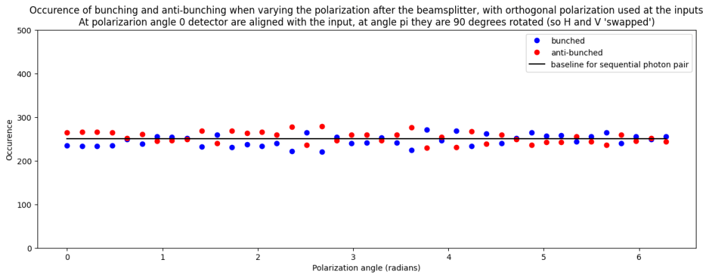
We can also change the polarization after the beamsplitter as in below illustration. In principle this also leads to ‘indistinguishability’, but then only after the photons have passed through the beamsplitter. What we will see is that the ration of ‘bunching’ and ‘anti-bunching’ is exactly as we would expect without quantum physics (so we do not observe the HOM effect in the beamsplitter, even though we make the photons indistinguishable before detection). What we do see is that we create ‘entanglement’ between the two photons when they end up in different ports, so still some very interesting quantum behavior to be observed!

When we look at the ratio bunching/anti-bunching we see in this case the same value as for sequential photon pair, so there is no quantum effect (even though we removed the photon distinguishability).

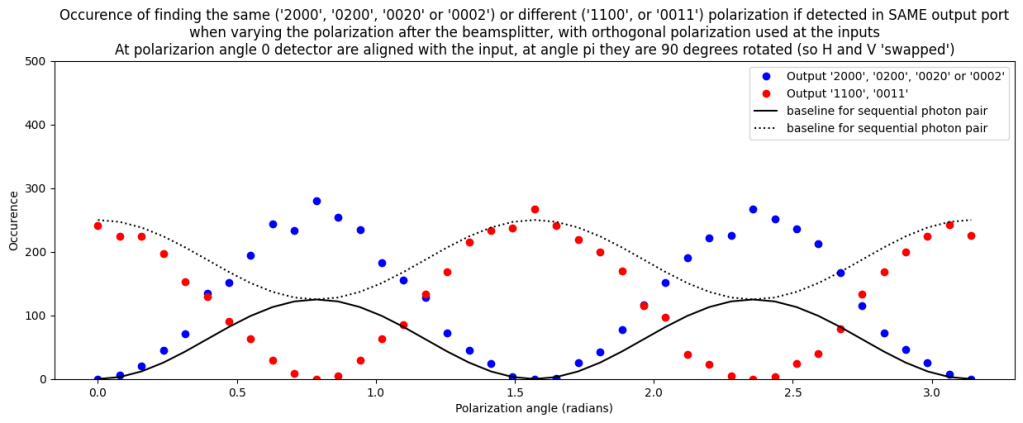
When we look in more detail we see interesting quantum effects. For instance when only looking at ‘bunching’ for certain orientation of the polarization after the beamsplitter we see that the occurence of detecting photons with different polarization is suppressed. So there is ‘bunching’, but only within the output port and not between the two output ports.

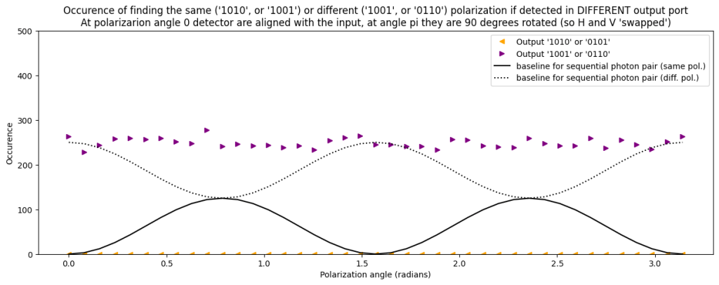
Another interesting effect occurs if we look only at the occurence of anti-bunching. Contrary to what we would expect we see that there is never a measurement outcome where the two photons end up in different port, with the same polarization. So if a photon behind port 1 is detected with horizontal polarization, then always the same is true for the photon in output port 2. Even though the actual detection of horizontal or vertical polarization is completely random.

Conclusion

In this notebook we played with a ‘simple’ beamsplitter and some rotation of the polarization. Even this system already shows intriguing quantum behavior with non-classical measurement outcomes and ultimately entanglement leading to non-local correlation. The assessment has been descriptive so far (we only looked at the outcome of the computer models). A next step would be to describe the beamsplitter more deeply and also model the quantum behavior mathematically.

The armchair quantum physicist