The armchair quantum physicist

See the Jupyter Notebook for the Quantum HOM Effect on Github pages.

Check out the previous post on the Quantum HOM Effect

Main reference: C. K. Hong, Z. Y. Ou, and L. Mandel, “Measurement of subpicosecond time intervals between two photons by interference”, Phys. Rev. Lett. 59, 2044 – Published 2 November 1987

Introduction

In a previous post we showed via computer experiments the ‘quantum behavior’ of a simple beamsplitter. If two photons entering the different ports of a beamsplitter are sufficiently ‘indistinguishable’ we see that the photons group together in one of the output ports (‘bunching’), while without quantum physics we would expect that in 50% of the cases we find one photon in each output port (‘anti-bunching’)

In this post we explore this effect deeper and try to describe it by simple mathematics. We will see that we in effect are looking at ‘quantum interference’ where the system can take different ‘paths’ to get to the same outcome. In quantum theory these paths can ‘interfere’, leading to the results we observe.

Results from computer experiments

In previous post we explored how varying the degree of ‘indistinguishability’ affect the occurence of bunching in the measurement results. We have used three methods to achieve this:

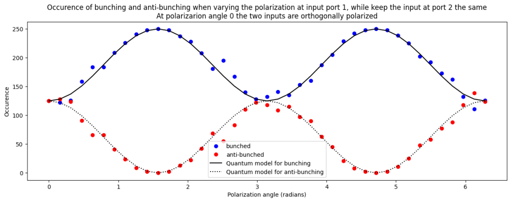
1. We rotate the polarization before one of the input ports of the beamsplitter. If the polarization for the two ports is parallel photons are ‘indistinguishable’, if polarization is orthogonal they are fully ‘distinguishable’.
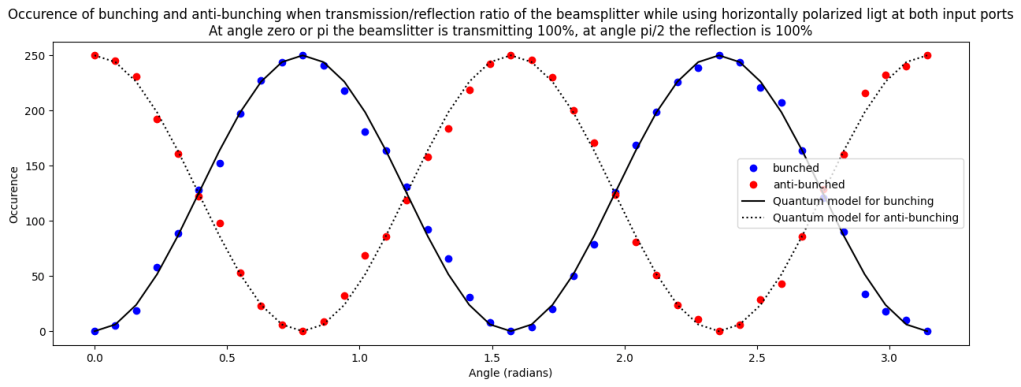
2. We vary transmission and reflectance of the beamsplitter and use photons with the same polarization at the input. If the transmittance is 100% the photons are ‘distinguishable’ (as they simply pass through and end up in a unique detector). If the tranmittance is 50% the photons are fully ‘indistinguishable’ as we are equally likely to see any of the input photons behind any output port.
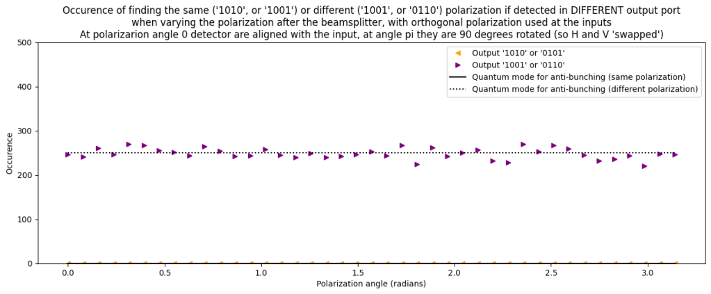
3. We rotate polarization behind the two ports of the beamsplitter. If we start with orthogonal photons and use a 50%/50% beamsplitter the photons are ‘distinguishable’ if we do not rotate polarization, but become ‘indistinguishable’ if we rotate polarization by 45 degrees.

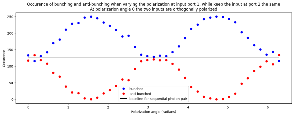
Varying the polarization at the input ports of the beamsplitter from orthogonal to parallel

In this case we observe that for orthogonal polarization at the beamsplitter input we see an equal amount of ‘bunching’ and ‘anti-bunching’. This is as expected without any quantum effects. If we rotate the polarization to parallel we see full bunching and the outcomes where we see one photon behind each output port are fully suppressed.

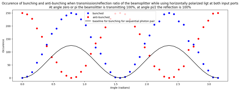
Varying transmission/reflection ratio of the beamsplitter

In this case we vary the transmittance of the beamsplitter and use parallel polarization at the input. Without quantum effects we would expect some variation in the level of ‘bunching’ (from 0% to 50% occurence), but in the experiment we see a more severe effect (swinging from 0% bunching to 100% bunching).

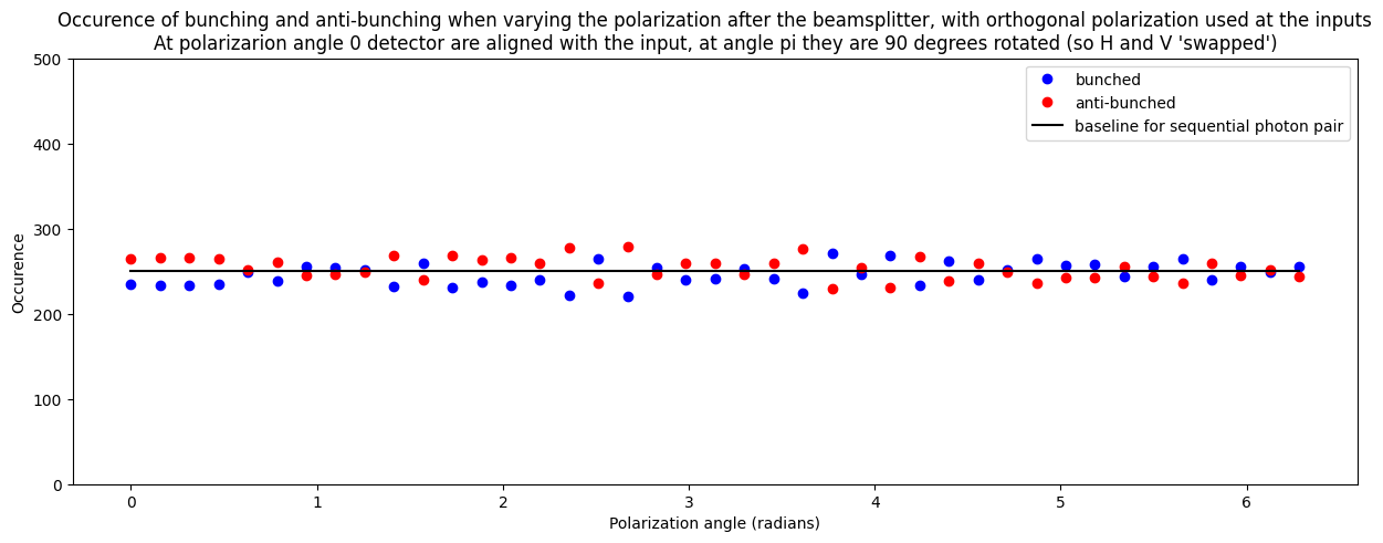
Varying the polarization after the beamsplitter

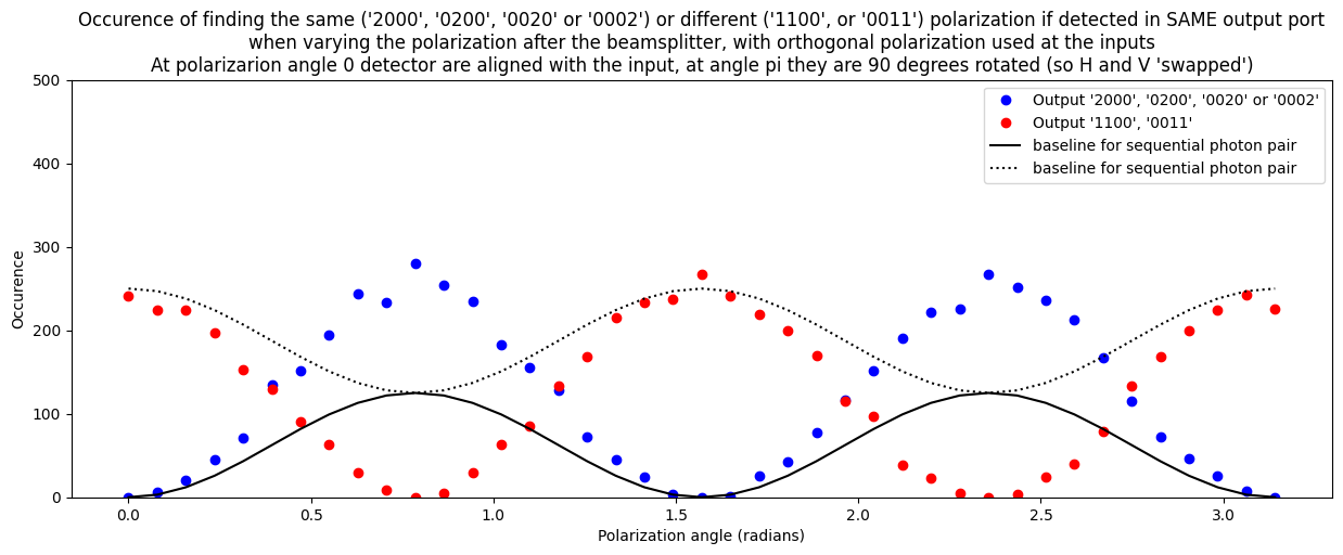
The last case we explore is where we adjust polarization AFTER the beamsplitter to vary ‘distinguishability’. Conceptually, if the driving factor for the HOM effect would be the level to which we can distinguish the two photons we would expect to see a full suppression of anti-bunching. This is however not what we observe. Even if we rotate polarization after the beamsplitter by 45 degrees we see the same occurence of bunching and anti-bunching. A closer look at the exact outcomes we see for bunching and anti-bunching however still leads to interesting results. For instance when the two photons end up behind two different output ports we see that they never have the same polarization. Somehow if the photon behind port 1 ‘decides’ to be horizontally polarized then the photon behind port 2 instantaneously ‘decides’ to be vertically polarized. This is an example of entanglement created by the beamsplitter, even though we did not have any entanglement in the input state.

Working with Fock states

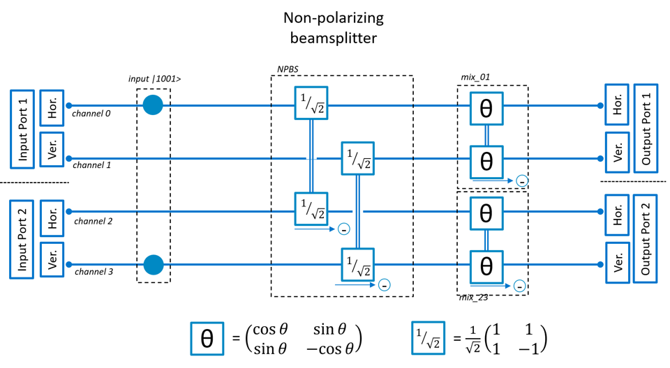
We use a beamsplitter with two input ports and consider vertical and horizontal polarization for each port. So we have 4 ‘channels’ in total. In the experiments we use one or two photons, so the maximum occupancy of each channel is 2. Hence we can describe the system with a 4 channel ‘Fock’ state. A Fock state is a quantum state where we can have a discrete number of particles. So each channel can contain 0,1,2,3, .. photons. Let’s have a closer look at the possible states for this system.

Single photons

If we have only one photon we can have the situation that this photon is uniquely in one single channel. For instance, for state |0001> we have a 100% probability of finding a photon in channel 3, so to detect the outcome ‘0001’. There is no ambiguity, we always get the same outcome and know exactly in which channel to find the photon.

Alternatively we can have the situation that we sometimes measure the photon in channel 1 (so detect the outcome ‘0100’) and sometimes in channel 3 (so detect the outcome ‘0001’). In that case the state would be α⋅|0001>+β⋅|0100>. We then have probability |α|² of detecting the photon in channel 3 (so detect ‘0001’) and |β|² of detecting the photon in channel 1 (so detect ‘0100’). Here |α|²+|β|²=1, as we need to have a 100% change of detecting the photon somewhere.

In this example we call |0001>and |0100> the components of the state. α and β are the amplitudes. Each component has a unique outcome for the measurement (like in this case ‘0001’ or ‘0100’. The probability to find a certain measurement outcome (‘0001’ or ‘0100’) is the square of the absolute value of the amplitude (so |α|² or |β|² ).

Two photons

For two photons in a state we have similar logic. Also here the state is build from components, with amplitudes and probabilities to detect a certain measurement outcome. Of course in this case we could detect two photons in a single channel.

For |0101> we have a 100% probability of finding exactly one photon in channel 3 and exactly one photon in channel 1. So we will always detect the outcome ‘0101’

For |0200> we have a 100% probability of finding two photons in channel 1 So we will always detect the outcome ‘0200’

In the above cases the states consist of only one component, which then has amplitude 1 and detection probability of 100%. For α⋅|0101>+β⋅|1010> we have probability |α|² of detecting the photons in channels 1 and 3 (so detect ‘0101’) and |β|² of detecting the photons in channels 0 and 2 (so detect ‘1010’). Here |α|²+|β|²=1, as we need to have a 100% change of detecting two photons.

Note that the probability is valid for detecting the outcome in full. If we detect a photon in channel 1 we will also detect a photon in channel 3. As there is no component for outcome ‘1100’ we will never detect a photon channel 0 and channel 1.

For α⋅|1001>+β⋅|1010> we have probability |α|² of detecting the photons in channels 0 and 3 (so detect ‘1001’) and |β|² of detecting the photons in channels 0 and 2 (so detect ‘1010’). As also here |α|²+|β|²=1 it means we always detect one photon in channel 0, and only see variation in the dection of the photon in channel 2 or 3. Note that although we have two components which have a photon in channel 0 we never detect 2 photons in this channel, |2000> is not a component so outcome ‘2000’ will not be detected.

Combining single photon states into one single two-photon state

Now we can try to ‘build’ two photon states from single photon states. Intuitively, we could predict from the single photon outcomes the probability for the two photon outomes. For instance, if we would have one photon in |0001> and another photon in |0100> the combined state woul be |0101> and we detect with 100% certainty the outcome ‘0101’.

Imagine now that we combine two photons with the states:  α1⋅|0100>+β1⋅|0001> and α2⋅|1000>+β2⋅|0010>. We then need |α1|²+|β1|²=1 and |α2|²+|β2|²=1. The final state is then α1α2⋅|1100>+β1α2⋅|1001>+α1β2⋅|0110>+β1β2⋅|0011>

In this example the likelihood of detecting one photon in channel 0 and one photon in channel 1 (outcome ‘1100’) would be |α1 α2|². It is easy to proof that |α1 α2|²+|α1 β2|²+|β1 α2|²+|β1 β2|²=1, so we are sure to detect any of the possible outcomes and will always find the two photons back in the measurement result.

The above result can be derived intuitively. The likelihood for detecting outcome ‘1100’ is |α1 α2|², which is the same as |α1|² |α2|². This ‘simply’ the multiplication of the probability of detecting the two photons in channel 0 and channel 1 for the single photon states. What is important is that for the combined state we multiply the amplitudes of the ‘single photon’ contributions to come to the amplitude of the ‘two photon’ outcome. The likelihood of detecting a specific ‘two photon’ outcome is then the square of this amplitude (or square of the absolute value of the amplitude if we take phases into account, for this post we can ignore this).

Including quantum effects

Now there are two important factors to consider in quantum theory, and these aspects break the ‘intuitiveness’ of the result.

Quantum Interference

One aspect is that in the final state there can be an ‘outcome’ which shows up multiple times with different amplitudes. There could for instance be a situation where either two photons are reflected by a beamsplitter, or two photons are transmitted by a beamsplitter both leading to the same detection outcome. In that case we have to add up the amplitudes for this outcome, before we take the square to calculate probability. If one of the amplitudes is positive, and the other is negative we have to in fact substract the amplitudes and the probability of finding this outcome will be reduced.

Imagine we have the component α⋅|0101> and the component −β⋅|0101>. In the resulting state we then have (α−β)⋅|0101>, with probability |α−β|². Note that this effect only takes place if the photons come together in the same state. If we would first detect one photon in state with component α⋅|0100> the probability of measuring outcome ‘0100’ would be |α|², for the second photon (arriving later) the probability of detecting |0001>would be |β|² (the minus sign disappears in the absolute value). There is no quantum interference in this case.

Boson bonus

One other aspect is that for photons (as for other bosons) there is a preference of grouping together in the same state. This means that if we combine two single states and the resulting state has a component where both photons are in the same channel (like |0200>), this component gets an additional factor of √2 in the amplitude. As example let us combine α1⋅|0100>+β1⋅|0001>, and α2⋅|0100>+β2⋅|0001>. The resulting state will have a component α1α2√2⋅|0200>, where the √2 is purely coming from the fact that there is a channel with photon number 2, i.e., a channel which is occupied by two photons. Would we have a situation where we combine three states we could end up with α1α2α3√3⋅|0300>, so the ‘bonus factor’ scales as the square root of the photon occupancy in the final state. Note that this effect only takes place if the two photons come together in the same state and are also detected in this state. If the photons arrive sequentially they would not group together, and the ‘boson-bonus’ would not be applicable

The two effects above lead to the situation that the probably of detecting a certain outcome deviates from what one would expect by looking at the two photons individually. The ‘quantum interference’ can only happen if the photons arrive simultaneously, and also the ‘boson-bonus’ is only applicable for two photons detected at the same time. Obviously in any case the probabilities of the different components have to add up to exactly 100% in order to ensure that we detect all photons that we put into the system also at the output (we ignore any photon absorption or creation). What we will see is that the ‘quantum interference’ and ‘boson-bonus’ work together to ensure this.

How to model the quantum effects

• We have states which consist of components. Each component has a specific measurement outcome. In the state each component has an amplitude and the probability of detecting the outcome related to a specific component is the square of the absolute value of the amplitude. As example consider the state α⋅|0101>+β⋅|1010>. We have probability |α|² of detecting outcome ‘0101’ and |β|² of detecting outcome ‘1010’. Here |α|²+|β|²=1, as we need to have a 100% change of detecting two photons. Detecting outcome ‘1010’ means we measure a photon in channels 0 and 2, and no photon in channels 1 and 3.
• The states can be manipulated by matrices, where the matrix components affect the amplitudes of the components. The matrices we use in this notebook are used for single photon states. If we have the matrix for a 2 channel system it works as follows on the single photon states and also  
• For states with multiple photons the outcomes at the output have an amplitude which is the multiplication of the amplitudes of the individual photons. As example if we ‘build’ a two-photon state with component |0110> from single photon states with amplitude α⋅|0100> and β⋅|0010> then the amplitude of the two-photon component is αβ⋅|0110>. The probability to detect the outcome ‘0110’ is then |αβ|²
• If the same component appears multiple time in the output it means there are multiple ways to get to that component (for instance two photons could pass through a beamsplitter, or two photons could be reflected to lead to the same end state). In that case we have to add up the amplitudes for these components if we detect the photons simultaneously. This can lead to quantum interference where a probability is reduced due to two amplitudes cancelling eachother for the different ways to get to an component.
• If a component has more photons in the same channel (so component  |0200>  or  |0030>) the component will get an extra multiplier in the amplitude of the square of the photon number. So for |0200> the boson bonus would be √2.

Modelling the impact of the quantum effects on the measurment outcomes.

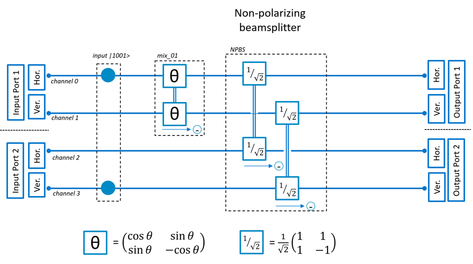
Changing the polarization of the input ports to vary ‘indistinguishability’

The photon which starts in channel 3 has two options. Either it will end up in channel 3 (i.e., pass through the NPBS), or it will end up in channel 1 (i.e., is reflected in the beamsplitter). In the first case the amplitude is −1/√2 and in the second case +1/√2.  So the state for that photon is 

If we would just use that photon the probility to detect it in channel 3 would be 50%, and the probability to detect in channel 1 could be 50%.

The photon starting in channel 0 has more options. It can end up in any of the channels at the output. First when we vary the polarization by ‘mixing’ channels 0 and 1 the photon can stay horizontally polarized and remain in channel 0. This gives an amplitude cos(Θ). If the photon is deflected to channel 1 (change polarization to vertical) the amplitude is sin(Θ). Then in each of these cases the photon either passes through the beamsplitter, or is reflected. This all with amplitude 1/√2. So the photon ends up in the state:

If we would just use this photon the probility to detect it in for instance channel 0 (outcome ‘1000’) would be .

Now we look at the two photons travelling through the system simultaneously. We then look at the amplitude of the single photons and multiply then to get to the amplitude of the corresponding component in the final state. This final state in principle has 8 components (two options for the photon starting in channel 3 multiplied by four options for the photon starting in channel 0).

First look at the outcomes where both photons end up with different polarization (so one horizontally and the other vertically polarized). We find that all these outcomes have the same probability.

So, in total the probability of finding an outcome where both photons have different polarization is .

Now lets look at the outcomes where both photons have the same polarization. As the photon staring in channel 3 will always remain vertically polarized we only have to look at both photons vertically polarized behind different ports (outcome ‘0101’), both behind port 1 (outcome ‘0200’) or both behind port 3 (outcome ‘0002’). Now we see the two quantum effects in action.

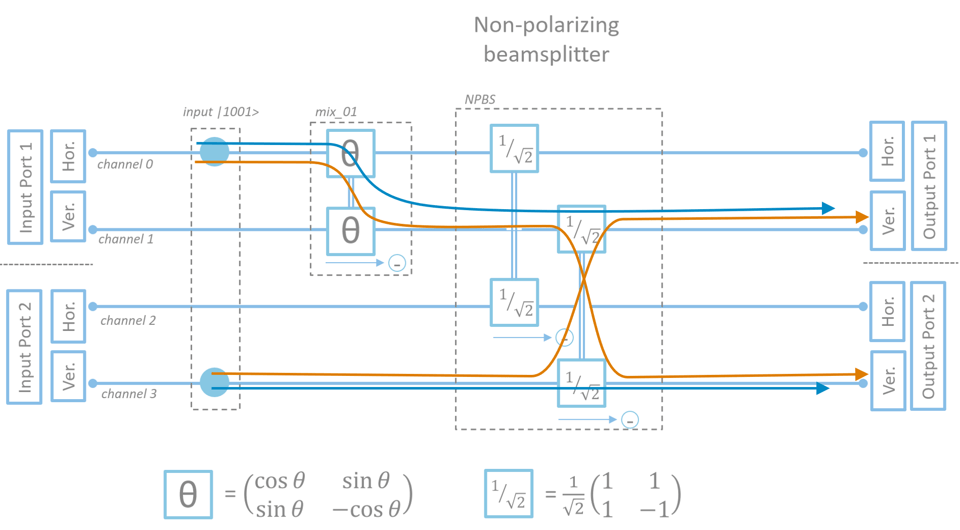
For the first case (outcome ‘0101’) there are two ways of creating it. We could have the photon from channel 0 end up in channel 1, and the photon from channel 3 remain in channel 3. We could also have the photon from channel 0 end up in channel 3, and the photon from channel 3 switch to channel 1. See the picture below for a graphical illustration. If we calculate the amplitudes for these different ‘paths’ we see that they exactly cancel when we add them up (one has a minus sign). Mathematically this is because only when the photon travels from channel 3 to channel 3 it picks up the minus sign. As the amplitudes are equally large, but with opposite sign they exactly cancel out. This is quantum interference in action.

For the components with two photons in the same channel we have to apply the boson bonus and add a factor √2. We nicely see that when we add up the probabilities for all possible outcome it is .

Now we can look at the measurements for ‘bunching’ and ‘anti-bunching’. For ‘bunching’ we add up the probabilities for outcomes ‘0200’, ‘0002’, ‘1100’ and ‘0011’. This is . For ‘anti-bunching’ we then add up the probabilities for ‘1001’ and ‘0110’, which is . All other outcomes have probability zero. Below we plot this calculated probability against the result of the computer experiment to see the perfect match.

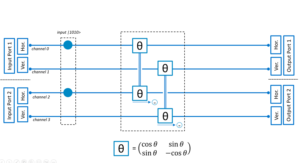
Changing the reflection and transmission of the beamsplitter to vary ‘indistinguishability’

In the case where we vary the reflectance and transmittance of the beamsplitter we can do similar analysis. In this case we have a photon starting in channel 0, which can either remain in 0 (with amplitude cos(Θ)), or be deflected to channel 3 (with amplitude sin(Θ)). The photon starting in channel 3 either remains in channel 3, with amplitude −cos(Θ) (note the minus sign!), or is reflected to channel 0 with amplitude sin(Θ). The components in the final state then look like:

Changing the polarization AFTER the beamsplitter to vary indistinguishability

For the case where we use polarization rotation after the beamsplitters single photons (starting in channel 0 or channel 3) can end up at any of the output ports with likelihood depending on the polarization angle. For the sign of the amplitudes we see that the photon starting in channel 3 can pick up a minus sign when passing through the NPBS, and when passing through the polarization rotators behind the ports.

For a photon starting in channel 0 (|1000>) the end-state is:

For a photon starting in channel 3 (|0001>) the end-state is:

From this we can assess the end state when we start with the two photon state |1001>. First look at the components with two photons in the same channel. The probability for any of these outcomes is the same (). The total likelihood of finding the two photons in one channel is  or

For finding the two photons behind the same port in different channels (i.e., with different polarization) the probabilities are calculated below. Each of these outcomes has likelihood , and for them together it is . What we see is that the total probability for a ‘bunched’ outcome is 50% as indeed we observe in the simulation. This is also the prediction without quantum effect (or the prediction for photon pairs that arrive sequentially).

Then we can look at anti-bunching where the two photons end up behind different ports. Logically the total occurence should be 50% (as the other 50% we should find a ‘bunched’ outcome). What is surprising is that the likelihood for finding the same polarization is zero. We only find antibunching with different polarizations! So while behind every port we find (for anti-bunching) a random polarization, of we compare the detection of horizontal or vertical polarization between the two ports we find a perfect anti-correlation. This is an example of entanglement, created from two non-entangled photons by means of a simple beamsplitter (so full linear optics) !!